RAM Parabolic Equation Code, Matlab Style

These are notes on using Collins' RAM PE Code for long range acoustic calculations. The specific package here is implemented in matlab as developed by Matt Dzieciuch. See also a comparison between RAM and Kraken.

Codes for Acoustic Propagation

RAM in Fortran 95. The suite of matlab scripts described on this page have been converted to Fortran 95 and parallelized using MPI.
RAM in Matlab. This page.
Eigenray A package for calculating acoustic rays and travel times by ray tracing.
Modes in Matlab. A simple matlab script for calculating acoustic modes by solving an eigenvalue/eigenfunction problem.

Table of Contents

RAM Parabolic Equation Code, Matlab Style

Downloads

aogpe.zip: Tar ball of code and mex files. Includes example run "peramx.m". (Updated 12/13/06)
sinc.m: The code requires the sinc.m file from the signal processing toolbox.
ram.pdf: Mike Collins' Documentation of the RAM Code (0.3 MB PDF file)
eflat.m: Flat earth transformation
eflatinv.m: Inverse flat-earth transformation
ridder.m: Used by inverse flat earth transformation

User Notes

Because the code is matlab, one can easily change it for whatever purpose one may like, and it is meant to easily integrate into a standard matlab working environment.

There is an example of how to run the code in a script called peramx.m. Using the mex files "solvetri" and "matrc" for your particular machine will make ram just as fast (or perhaps a little faster) than the original fortran version.

J.C.: One good test I have found in a pe code is whether it propagates a mode without introducing numerical coupling; I'll try that on your RAM for various grids. M.D.: I have done the test of propagating a high angle mode with ram and it seems to work. As you say, this is a good way to check if the grid size is adequate.

Comments on Accuracy

Subject: Re: RAM Matlab Code

Brian, It was not my intent to alarm everyone, but the details of range dependent modeling in acoustics is still a research issue. Even Mike Collins would agree. My only suggestion is to make comparisons among the various versions of RAM, i.e. different Pade coefficients, and make comparisons to CSNAP and other range coupled normal mode codes.

b/r, Arthur [Baggeroer]

Subject: RE: RAM Matlab Code

Art and Brian - Yes, I would concur that this business of modeling range dependent environments can get tricky, especially when the range dependence is small scale like internal waves. Often I have found that one's confidence in a model increases when multiple models show the same results, like coupled mode and PE showing agreement. When Andrey showed agreement between our PE Monte Carlo calculations and the coupled mode theory to within 3 dB at 2000 km range I was tremendously impressed.

Best,

John [Colosi]

Parameters

Accurate calculations depend on a number of parameters, and as always there is a trade off between speed and accuracy. It is also true that phase errors accumulate, so if a grid is good at 100 km, it may not be good at 1000 km.

np: The number of pade coefficients. The calculation is not very sensitive at all to to this number, and np=4 always seems to be a good choice.
deltaz: The depth increment for the PE grid. Picking the correct grid size for ultimate speed is important. While a coarser grid is faster, it will not be as accurate. A deltaz=1.0 is O.K., while a deltaz=0.2 will produce more accurate results but take an order of magnitude longer to complete. This value is also dependent on frequency, with higher frequencies demanding smaller values. For fc=250 Hz, deltaz=0.2 is probably closer to what is needed. A calculation at ca. 1500 km range and 75 Hz required a deltaz of 0.5 for an accurate result; deltaz=1.0 resulted in 10-20 ms increased dispersal of the arrival pattern.
deltar: The range increment for the PE grid. The code is less sensitive to the range step, but this value should be set small enough so that the PE converges. Also, N*deltar should equal the sound-speed horizontal sampling distance, where N is an integer. So if you've used a sound speed grid of 1000m, deltar=250 should work, but if you use a sound speed grid of 400m, then set deltar=200m. The value of deltar is inversely proportional to computation time.
T: The time window. This value sets the width of the time window for the calcuations. The value of this window sets the number of frequencies that are required to do the calculation, hence it is directly related to the computation costs. The value should be tuned to the expected dispersal of the arrival pattern. Too large a value just means that more frequencies than needed have to be calculated.
dzm: The depth interval used for output depth decimation. This number is not related to the calculation, per se, but is related to how coarsely the results are subsampled for plotting. Too small a value results in a grainy looking figure.

fc: The center frequency desired. 75 Hz for ATOC-like transmissions, 250-Hz for HLF-5-like transmissions.
fs: Sample frequency, generally 4X the center frequency.
N: The number of frequencies for the calculation=fs*T. (not a user specified parameter, except through T.)
df: The frequency increment=fs/N. (not a user specified parameter, except through T.)

tdelay: The time delay, which sets the start time for the window of width T. This value should be roughly the range divided by a nominal sound speed, c0. c0=1485 or 1490 m/s. The value of tdelay is used to place the prediction in the correct (unaliased) time window.

attn: Attenuation. The default attenuation is 0.5 db/wavelength 100m below the bottom, and 5db/wavelength 300m below the bottom. Bottom reflections are/were discouraged in this code. Attenuation is a two row matrix, the top row being attenuation 100 m below the bottom (0.5), the second row row being below that (5). The exact parameterizations vary wildly in the actual ocean, and are poorly modeled, in any case. The default choices for sediment density and speed are unrealistic, but since the attenuation is so high one wouldn't notice. A somewhat more realistic WAG (Wild Ass Guess) as opposed to the SWAG (Stupid Wild Ass Guess) that I used might be rho=1.1 kg/l, cs=1700 m/s.

Mex file compilation

The package includes two C routines, matrc.c and solvetri.c, that should be compiled to obtain mex-files for these functions. These routines will allow the RAM code to run more than an order of magnitude faster. There are two ways to compile these routines:

Place the file "mexopts.sh" in the local directory and edit it for your own situation. The file has sections for x86, xa64, and solaris architectures, and matlab will automatically select the correct architecture for the computer you are on. Set CC, CXX, or FC to be your C-compiler, C++-compiler, or FORTRAN compiler, respectively. You can, in addition, set whatever optimization flags there (e.g., "COPTIMFLAGS") you'd like to try. With that file in the local directory, "mex matrc.c" will compile the mex file, using the options in this local file (otherwise it uses the default version in matlab's installation directory). Use the "-v" option, if you want to see what is going on.

Matt D. has put together a makefile that is also suitable to compile the mex files. Edit this file to set your compiler and optimization flags, and then execute "make all", which should compile the mex files and link in the appropriate libraries. This makefile is set up for the x86 architecture, and it will require significant modification to work on the xa64 architecture.

Portland group compiler options include "-fastsse -tp p7", while gnu compiler options include "-O3 -mfpmath=sse -msse -march=athlon-xp", or "-O3 -mfpmath=sse -msse2 -march=k8" for AMD64 cpus. In linux, "cat /proc/cpuinfo" will tell you what SSE support your cpu has. "Your mileage may vary."

Range Dependent Sound Speed

Range dependent sound speed is implemented by defining variables:

rp - ranges of profiles in meters
nrp - number of profiles
cw - matrix of sound speeds Each row is a sound speed profile.
zw - depth of sound speeds in meters (positive down)

In general, I think it is true that the zw have to be at a fine increment of O(1m), and the same zw should be used for all profiles. Adding range dependence will make the code run considerably slower. The following segment of matlab code will produce values appropriate for ram from the sound speeds derived from the matlab mapping package. The mapping package extracts sound speed from the WOA on 33 standard depths.

load temp.ssp I=(temp(:,1)==-1); rp=temp(I,2)*1000; nrp=length(rp); 
zq=temp(2:34,1); cw=temp(:,2); cw=reshape(cw,34,nrp); cw(1,:)=[]; zw=0:1:5000; 
zw=zw(:); cw=interp1(zq,cw,zw,'spline');

cw is a matrix, while rp and zw are a vectors. While it is not strictly necessary to interpolate sound speed to the zw, you should interpolate on your own. RAM will just linearly interpolate sound speed to the grid size specified to deltaz. A coarsely sampled sound speed could therefore lead to biases, false caustics, war with Iran, etc.

The source depth, sound speeds and depths require the flat-earth transformation before sending to RAM (see also downloads).

% Flat earth transform: Re=6378137; invRe=1/Re; eps=zw*invRe; 
zw=zw.*(1+(1/2)*eps+(1/3)*eps.*eps); eps=eps*ones(1,nrp); cw=cw.*(1+eps+eps.*eps); 
cw=cw';    % ram expects sound speed profiles in rows.  eps=zsrc*invRe; 
zsrc=zsrc*(1+(1/2)*eps+(1/3)*eps*eps);

To include the effects of internal waves in this calculation, sound speed has to be defined on fine enough depth and range increments to resolve the internal waves of interest. This makes cw a rather large matrix.

Range Dependent Bathymetry

Implementing range-dependent bathymetry is easy. The code just needs vectors "rb" and "zb", which are the bathymetry ranges and bathymetry values (both in meters), respectively, along the path of interest. The bathymetry extracted using the mapping package can be loaded in by the following simple matlab code:

load temp.bth rb=temp(:,1); zb=temp(:,2);

Adding bathymetry, other than flat bottom, to the calculation will slow it significantly - by a factor of 5 or more. matrc needs to run every time there is an environmental change (sound speed or bathymetry), so the rough bottom case will take longer than the flat bottom case.

Parallelization Notes

The computations involve completely separate calculations at the different frequencies of the broadband signal, hence the parallelization problem in this case is trivial. One need merely farm out various sets of frequencies to whatever computers one has available, let them run their calculations, and then collect the results at the end. The code has an implementation of parallelization using matlab's tcpip toolbox already implemented, but there are other ways to do this.

The parallelization just has to fill the columns of the matrix psif. So, one way to parallelize the calculation would be to have each processor fill different columns, and then collect the results after they are all done.

FAQ

Can this RAM do 3-D? RAM cannot do azimuthal coupling although the scaling is set up for a 3-d non-coupled problem.
The final figure is rather grainy. How would I boost the resolution of the arrival depth-travel time figure? You probably have the decimation factor, dzm, set higher than you'd like. The output grid size is dzm*deltaz.
How come the travel times predicted by RAM are way off compared to a similar ray prediction, yet the arrival patterns are the same? The RAM code makes a prediction for a time window "T", and that time window is aliased infinitely many times. Therefore, you need to apply a reasonably accurate time delay to put the time window "T" in the physically correct time. This involves giving the code a reasonably accurate value for "tdelay", which roughly the range divided by a nominal sound speed. For the Pacific, a nominal sound speed is ca. 1485 m/s, while a larger value is more appropriate for the Atlantic. The travel times predicted by RAM are correct, if you set the time window such that the physically correct arrival pattern (rather than an alias) appears in it. It is helpful to compare the RAM result to a ray prediction to be sure a good value for the time delay is being used.
How come the travel times predicted by RAM are way off compared to a similar ray prediction? The RAM code uses the unmodified sound speed that is input to calculate the propagation, whereas most ray codes (e.g., eigenray) apply a flat-earth transformation before calculating the propagation. The flat-earth transformation accounts for the spherical earth; sound speeds and depth are stretched slightly to be equivalent to propagation on a sphere. So try applying the flat-earth transformation to your sound speeds before doing the RAM calculation (see eflat.m download above), or turning off the flat-earth transformation of your ray code, if you can.

Benchmarks

Matt's unadulterated test case (peramx.m) is used for these benchmarks. This test case is 100-km propagation of a broadband signal in a range independent ocean given by the canonical sound speed profile. Time uncertainties are ±1-2 s.

Processor	<Details	Time	Notes
Intel Q6600 Quad Core	o'clocked to 2.8 GHz 2X2MB L2 cache	13 s.	Intel icc compiler; "-fast"; single proc.
Opteron Dual Core 265	1.8 GHz, 64 bit 1 MB L2 cache	30 s.	"-O3 -msse3 -march=opteron"
Opteron Dual Core 265	1.8 GHz, 64 bit 1 MB L2 cache	Two procs 31 s.	"-O3 -msse3 -march=opteron"
Opteron Dual Dual-Core 265	1.8 GHz, 64 bit 1 MB L2 cache	Four procs 36 s.	"-O3 -msse3 -march=opteron"
Athlon 3200+ 64	2.0 GHz, 64 bit 1 MB L2 cache, laptop	33 s.	"-O3 -mfpmath=sse -msse2 -march=k8"
Athlon 3200 XP	2.2 GHz, 32 bit 512 KB L2 cache	47 s.	"-O3 -mfpmath=sse -msse -march=athlon-xp"
Athlon 2500 XP	2.0 GHz (OC'd), 32 bit 512 KB L2 cache	60 s.	"-O3 -mfpmath=sse -msse -march=athlon-xp"
Xeon	2.2 GHz, 32 bit 512 KB L2 cache	61 s.	pgcc: "-fastsse"
Athlon 2000 XP	1.6 GHz, 32 bit 256 KB L2 cache	81 s.	"-O3" (old gcc; minimal options)

Solvetri.c is compiled to the mex file with the options as indicated. The mex file for the matrc routine improves computation time by a factor of 2 (more for longer range computations) or so.

Benchmarks in practice... Calculating PE predictions for an acoustic path in the Philippine Sea for 36 ECCO2 ocean model realizations. Time listed is for a single frequency. All values "under load", that is, all cpu's running. Using the 80 cpus of aogreef, the 36 snapshots at 628 km range took about 10 hours total (72sX13 frequencies for each cpuX36 realizations=9.4 hrs.) All calculations used the mex files compiled with the GNU gcc. It appears that the Intel icc compiler might gain an additional 7% or so. compiler with "-fast" option.

Processor	Details	Time	Notes
Phenom 9600	2.3 GHz, 64 bit 4X512 KB L2 cache	Four procs 50 s.	bluefin
Intel Q6600 Quad Core	o'clocked to 2.8 GHz 2X2MB L2 cache	Four procs 57 s.	skipjack
2×Opteron Dual Core 265	1.8 GHz, 64 bit 2X1 MB L2 cache	Four procs 72 s.	sardines
Opteron Dual Core 170	2.0 GHz, 64 bit 2X1 MB L2 cache	Two procs 73 s.	anchovies
2×Opteron Dual Core 2210	1.8 GHz, 64 bit 2X1 MB L2 cache	Four procs 75 s.	aogreef

References

M. D. Collins, A split-step Padé solution for the parabolic equation method, J. Acoust. Soc. Am., Vol. 93, pp. 1736-1742, 1993.
M. D. Collins, An energy-conserving parabolic equation for elastic media, J. Acoust. Soc. Am., Vol. 94, pp. 975-982, 1993.

Figures

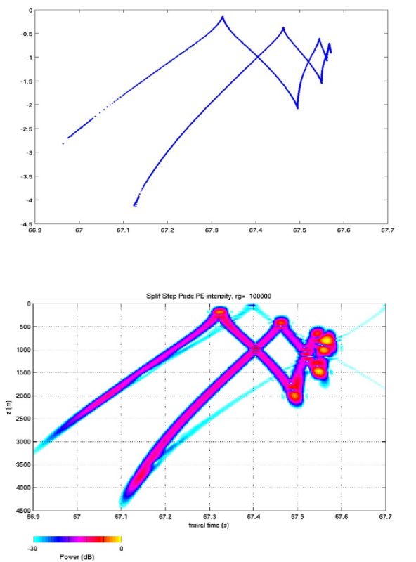
Comparison between Eigenray prediction and RAM prediction for 100 km range (NOT the test case!)

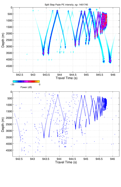
Comparison between Eigenray prediction and RAM prediction for 1401.745 km range. This comparison shows the effects of bathymetry in the form of a sharp ridge midway along the acoustic path. The comparison illustrates two problems that can be fixed by adjustment of the calculation parameters. (1) Note that the ray and PE predictions shown here have slightly different dispersal, which is particularly evident in the early part of the timefront. This is the result of using too large a value for "deltaz". When deltaz=0.5, rather than 2.0 (as was used here), this discrepancy is resolved. (2) The odd arrival in the lower right hand corner of the PE prediction is a result of using too small a value for T - the window is not wide enough so the earliest arrival appears to overlap the finalé. A larger value for T will give a window wide enough to encompass the complete arrival pattern with no wrapping around.