MPIRAM: The RAM Parabolic Equation Code in Fortran 95These are notes on using a version of Mike Collins' RAM PE solution for long range acoustic calculations. The specific package here is implemented in Fortran 95. It is directly derived from the matlab code developed by Matt Dzieciuch; indeed matlab and Fortran 95 are so similar, most of the adaptation to Fortran was just copy-paste from the matlab. One of the main goals of the Fortran approach was to parallelized the calculation using the Message Passing Interface (MPI) standard, hence this package of Fortran code is named MPIRAM.
Codes for Acoustic Propagation
Table of Contents

Downloads
Motivation
There are three main reasons for adapting the matlab code to Fortran.
The first reason is the suspicion that a Fortran version of the code
would run faster than a matlab version, and indeed benchmarks suggest
the Fortran implementation is some 25-30% faster, depending on the
compiler. The second reason is that the parallelization problem is
easier to deal with in Fortran, in this author's opinion, since the
suite of communication subroutines from MPI can be easily employed. The
parallel version of this code is quite easy to manage. And the third
reason is to give some flexibility to adapting the code to other
implementations, e.g., the possible use of Cuda Fortran 95 was used because this user is most familiar with Fortran; matlab code is astonishingly similar to Fortran 95. In addition, Fortran 95 allows for arrays to be allocated on the fly to any size, which is a very convenient feature. This code is designed to run with the suite of subroutines from the "Message Passing Interface" system (MPI) on a cluster, hence its name, MPIRAM. There is a single processor version for simple situations, however.
Single/Double PrecisionIn June/July 2013, I learned that there is no inherent reason why RAM, or PE calculations in general, should be all in 100% double precision (Kevin Heaney, Kevin Smith, Richard Campbell, Mike Porter, to name a few who confirmed this...). A few reconfigurations later produced mpiramS, the single precision version, which works very well for computations out to a few megameter range. It developed that for small deltaz, required for an accurate prediction of time fronts, some pesky numerical noise arose. This noise was traced to variables in the subroutine matrc, so that the new code is set up to be mostly single precision, with double precision used for key elements. The documentation for RAM by Collins notes this. Using mostly single precision gives calculations adequate for most cases, at about half the computational cost. In addition, intel's hyperthreading technology becomes very effective with this single precision code - going from 4 CPUs to 8 hyperthreaded processors gives a ca. 40% boost in computation. One can convert this code to 100% double precision by editing the src/kinds.f90 module and changing the precision for "wp" to "kind(1.0d0)". Change the reads of the matlab script plotram.m to real*8 from real*4 as well. Or change to 100% single precision by changing the precision for "wp2" to "kind(1.0e0). With this reconfiguration, the requirement for lapack/blas elements was discarded in favor of the original gaussian elimination subroutine employed by Collins. The code was also redesigned slightly to allow for parallelization using openmp. One can now use either openmp or MPI. The MPI version seems to run slightly, 4%, faster on a single CPU. MPI also allows many computers to be brought to bear on the task. Note that changing the precision to all double precision requires changes to the MPI calling routines in peramx_mpi.f90 to MPI_Double_Precision rather than MPI_FLOAT or things will crash.
PhilosophyThis code, and the other codes for acoustic propagation listed at the top of this page, is designed for deep-water, long-range, low-frequency, broad-band acoustic propagation. The codes may well work for shallow-water, short-range, and high frequencies, but the author of this code makes no representation that it is good for those situations. You should be approaching this code with the notion that you will be adapting it to suit your own specific purpose. There are too many complicated issues involved with calculating acoustic propagation with the RAM code to be able to put together a one-size-fits-all suite of code. Issues range from whether internal waves are being modeled or not, which affects the spatial resolutions implemented in the code, to whether and how bottom interactions need to be modeled, which is beyond the scope of this small page. So, this code should be viewed as a set of parts, put together in some generic, example-type way, that you will need to tune to your own needs. Because the Fortran 95 coding is similar to matlab, it should be easily adaptable to a specific purpose. The output from this code is also designed to easily integrate into a standard matlab working environment; a matlab script to read the direct binary file written by the code is provided. The design of the code makes use of Fortran 95 modules to define common areas of data that are shared between the main program and its subroutines. These modules take the place of COMMON blocks of FORTRAN 77, but are far easier to deal with. These modules are: envdata.f90, mattri.f90, param.f90, and profiles.f90. The effect is that one does not have to pass variables to subroutines in long lists; rather, the data are available already to the subroutine. kinds.f90 and interpolators.f90 are also modules, but they are used for other purposes.
Compilation NotesCompiling the code should be relatively straightforward - the code has compiled successfully on g95, gfortran, Intel's ifort compiler, and the Sun Studio compiler. (Of these the Sun compiler produced the fastest executable for the longest time, but gfortran 5.0 now seems to be the best one to use.) Makefile's are provided for all components of the code. The first task is for the user to take a look at the Makefile's and edit them for their intended compilers. Compiling LAPACKThe code need to solve a small matrix problem in epade.f90. In older versions of the code, LAPACK routines were been set up to do that. Either a standard LAPACK library can be linked to the code, or, for portability, the small subset of LAPACK routines needed to do the calculation are included in the tarball in the subdirectory "lapack". Executing "make" in that directory should produce an archive smlapack.a (for "small lapack") that can be linked to the code. This is a very small calculation; efficiency is a non-issue here. This requirement is not needed with the more recent mpiramS. Compiling MPIRAM - single processorJust executing "make" should make the single processor binary, with the resulting executable s_mpiram, for "single mpiram". "make clean" will delete the object (./obj/*.o) and module (./mod/*.mod) files. With the more recent mpiramS, this compilation can employ openmp to bring multiprocessor CPUs to bear on the task. Compiling MPIRAM - MPI processingThe first step to compiling MPIRAM to do calculations in parallel is to install MPI, configuring it to use a Fortran 95 compiler. A description of how to do that is beyond the scope of this document. "See Also" below gives a link to the MPICH implementation of MPI. The Makefile for the MPI version is "Makefile.mpi" - take a look at this file to adjust the various compiler flags and lapack library for your own situation. The compiler to use is "mpif90", which is a product of your MPI installation and the compiler you configured it to use; the compiler flags in Makefile.mpi should be tuned to your Fortran compiler. Then "make -f Makefile.mpi" should compile the modules and code and produce the mpiram binary
The Input File: in.peA prerequisite to putting together a reasonable input file is the documentation on the various parameters given on the RAM in Matlab page. Critical parameters are T (time window), deltar (range increment), and deltaz (depth increment). The discussion of the nature of the parameters will not be repeated here. When the binary runs, it takes no input from the console, but looks for a file "in.pe" to read in the parameter and filename information it needs. Here is an example: Example in.pe File ! input file to PE - CAUTION: formatted input! 75 2 ! center frequency (Hz), fc, and Q value; bandwidth=fc/Q 2.0 ! time window width (s) - expected arrival pattern duration 1000.0 ! source depth (m) 30000.000 ! receiver range (m) 0.5 ! deltaz - an accuracy parameter (m) (0.5 is liberal) 250.0 ! deltar - an accuracy parameter (m) (250 is liberal) 4 1 ! np-# pade coefficients, ns-#stability terms 10000.0 ! rs - stability range (m); ns=0 for shorter ranges 50 ! output depth decimation (integer) (decrease if you get ripples in your matlab plots) test.ssp ! Input the soundspeed filename (for single processor, use "munk" for munk canonical) 1 ! Flat earth transformation: 0=no, 1=yes 1 ! Horizontal linear interpolation flag: 0=no, 1=yes 0 ! Enable ocean bottom? 0=no, 1=yes (yes turns on reading the file) test.bth ! Input the bathymetry filename (not used if ocean bottom = 0 above) 1 ! Flag for node weighting when computing on a cluster. Set to 0 to evenly weight. nodewts.dat ! File name for node weights (not used if flag is 0). The user should adjust these parameters for his own circumstance, taking care to respect the format of the file. ( To enable the comments on the right, formatted input is used - keep the same number of decimal places in the numbers and don't let the exclamation marks get too far to the left, where they might be picked up by the code.)
Running MPIRAMTo run the single processor version of mpiram just execute the binary ./s_mpiram. It will read the in.pe input file, do the calculation, and write out two files: psif.dat a direct access binary file with the results and recl.dat which stores the value of the record length of the direct access file in ascii. The latter is needed to be able to properly read the binary file later.
Running the MPI binaryFirst, be sure to copy the mpiram executable binary to all the remote locations, to a location that is in your search path; I like to copy it to /home/yourusername/bin/. On the aogreef.ucsd.edu cluster, the filesystem is mounted NFS so the binary is available to all nodes by default. To run the MPI version of the binary, the code needs a bit of a wrapper around MPI: time mpiexec -n 11 time mpiram will run the mpiram executable on 11 nodes and time the execution on each node and for the job as a whole. As for the single processor version, mpiram will read the in.pe input file. The convenient script runit is provided that contains this line. <Control>-<c> will abort the job on all nodes, if necessary. As for the single processor version, the code will write out two files on completion of the calculation: psif.dat a direct access binary file with the results and recl.dat which stores the value of the record length of the direct access file in ascii. For small values of deltaz on an SMP machine, the calculations do not seem to scale well with the number of CPUs, and one might be better off running fewer jobs than there are CPU's. On my quad-core systems, 3 jobs per system is more efficient than 4; it can take a bit of experimenting to settle on the optimal configuration. Load balancingThe last entries in the "in.pe" file allow the calculation to assign blocks of frequencies based on the computational ability of each processor of the cluster. This is useful if one has an eclectic cluster consisting of older and newer processors. Set the flag to be 1 for the code to read in the weighting values from a file, or 0 to just assign equal number of frequencies to all. To assign the weights to each node, just use the time required to calculate a single frequency as reported by mpiram (See "Benchmarks" below). The code will then do a simple calculation to assign more frequencies to faster processors. One can optimize the calculation by fiddling with the numbers to assign more or fewer frequencies to each node. Here is an example of an input file: 56 % Four cpus of node 1 56 % Set the value to be the approximate compute time for one frequency. 55 55 87 % Four slower cpus of node 2 87 % mpdtrace gives the order of the nodes 87 87 54 % Four cpus of node 3 54 55 55 45 % Two faster cpus of node 4 (a quadcore Q6600 that does not scale well to four processors) 45 The order of the nodes is as reported by "mpitrace -l". mpiram will write out the node names and number of frequencies assigned to each. The user should check that the number of frequencies are assigned to the nodes in the right order.
Working With the Results in MatlabWe live in a matlab world these days, and the MPIRAM source code distribution includes a small matlab script "plotram.m" that will read and plot up the results of the calculation. Most of that script has been borrowed from Matt's matlab version. The results of the calculation are written as direct access binary file, and they include a collection of essential parameters (frequency, time window width, Q, etc.) and the complex full acoustic field. To read the direct access file, the matlab script first reads the file written by MPIRAM named recl.dat, which has the size of the record length of the binary file. It develops that this number is not the same among different compilers, e.g., for the intel compiler it has to be multiplied by a factor of 4 for the matlab reads to work properly. So getting the correct correspondence between the MPIRAM and matlab record lengths may take some minor fiddling.
Input Sound Speed: Vertical and Horizontal InterpolationIt can't be stressed enough that the user should be responsible for giving this code sound speed realizations that have adequate, accurate resolution to begin with. The code does some interpolation, i.e., has a certain model for how to treat horizontal and vertical variations, but that treatment should not be relied upon for accuracy. For calculations involving fine-scale variability, e.g., internal waves or sharp ocean fronts, the sound speed sections input to the code should have the appropriate horizontal and vertical resolution to begin with.
Horizontal InterpolationThe RAM model has no inherent way to treat range dependence. When the code is given a range-dependent sound speed section, it just marches along in range, taking the nearest sound speed profile. If coarse resolution sound speed are given to the code, rather dramatic results make arise from possible abrupt changes to the sound speed profile as the code jumps from one profile to the next. In effect, such abrupt changes may lead to aggressive and unphysical mode coupling. Short of sending the code adequate sound speed sections, the Fortran 95 version of the code will optionally perform a linear interpolation of the sound speed section horizontally to make the changes to the sound speed profiles more gradual. The model in mind here is if one wanted a quick PE calculation using a section derived from the World Ocean Atlas. If you wanted none of this horizontal interpolation, you may change the flag in the input file to turn it off. If you wanted the code to calculate horizontal resolution differently, then change the relevant code in the peramx.f90 source code.
Vertical InterpolationThe RAM propagation technique needs to interpolate the sound speed onto a depth grid with spacing deltaz. The original version of RAM, including the matlab version, did this interpolation by linear interpolation in the "gorp" function. This simple interpolation made it essential to input fine-scale sound speed profiles to the code. For ranges O(1000 km) a value of deltaz of 0.25 m or less is appropriate, hence the vertical interpolation is to very fine scale, indeed. For little additional computational cost, the Fortran 95 version of the code implements a cubic spline interpolation onto the deltaz grid. For the same input sound speed section, this author believes the cubic spline approach will be slightly more accurate. At the same time, for simple calculations such as sound speed sections derived from the World Ocean Atlas, this Fortran 95 version of RAM will give a fairly accurate result even if coarse-resolution sound speed profiles are input. Similarly, the vertical resolution of the input sound speeds can be irregular, perhaps with high resolution near the surface, and lower resolution deeper. Considerable memory is also saved, since sound speeds with superfine resolution throughout the water column are not required. However, it is stressed again that this interpolation inherent in the model should not be relied upon to give accurate vertical interpolation - rather, the interpolation should be viewed as just part of the machinery to do the calculation. Be sure to give the code adequately resolved sound speed profiles, and bear in mind that the code will be doing a cubic spline to achieve the deltaz -spaced grid.
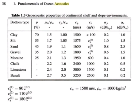
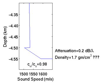
Notes on the Sea FloorThe code implements a very simple model for the ocean bottom and the acoustic interaction with it. No shear is modeled, and acoustic energy that interacts with the bottom is rather excessively attenuated (0.5 dB/wavelength). The code is generally designed for ocean-only propagation. Nevertheless, there are situations when it would be helpful to have some notion of what bottom reflected energy might look like, and this code might be able to do that. For more accurate calculations involving the ocean bottom, there are other versions of RAM that might be more appropriate (RAMGEO or RAMS).
Again, this model, together with parameters such as attenuation and density, needs to be adjusted from their nominal values to something suited to the user's purpose. Alternatively, the model for the sea floor may be entirely rewritten by the user, perhaps to include range-dependent sea floor properties read in from a data file. The code author is no expert in bottom interaction! Since following the bathymetry requires that the code continuously update the various matrices inherent to the calculation, turning on variable bathymetry makes the calculation take considerably longer (several times longer) than the flat bottom case. The subroutine matrc.f90 is called whenever there is a change to the environment.
Processor Benchmarks
Compute time for mpiram at 3 Mm range The benchmark cited is the time to complete one frequency; each processor works on only one frequency at a time. To compute the time to complete the entire task take the number of frequencies (749 in this case), divide by the number of processors employed, and multiply by the benchmark time. For example, on the Q6600 using four processors and the older version of mpiram would take: (749/4)*125 s=23406 s, or 6.5 hrs, but using only two processors it would take only: (749/2)*38.7=14493s, or 4.0 hrs. The new "hybrid" single/double precision version scales much better on SMP machines, including making effective use of hyperthreading and maximizing the performance of the AMD 8-core processor. Mpiram scales perfectly across the nodes of a cluster; it has minimal inter-computer communication. The compiler used here is gfortran 5.0 with general option "-Ofast -march=XXXX"; gfortran 5.0 appears to compile noticeably faster binaries than older versions. The MPI version employed because it is a several percent faster than the OMP version. Faster RAM settings can greatly improve performance, if you can get them stable.
† N.B. : When benchmarking, beware the powersavings mode! Mpiram seems to get its timing from the initial frequency of the CPU, so starting from a CPU in a low-frequency power savings mode and using an older linux kernel will give timing errors of a factor of 2 or so. When timing, it may be better to get the CPU's spun up to maximum somehow before starting mpiram.
See Also
Copyright © 2008-2015 by the contributing authors. All material on this collaboration platform is the property of the contributing authors. | |||||||||||||||||||||||||||||||||||||||||||||||||||||||||||||||||||||||||||||||||||||||||||||||||||||||||||||||||||||||||||||||||


