The Eigenray Acoustic Ray Tracing CodeThis is a page to download the source code for the "eigenray" ray propagation code for calculating the basic properties of rays over long ranges in deep water. Other hints for using this code and benchmarks can also be found here.
Codes for Acoustic Propagation
Other formulations/code for running acoustic ray calculations in the oceans can be found here: http://www.hlsresearch.com/oalib/Rays/index.html Table of Contents
DocumentationEarly in the development of the source code, I wrote a short Technical Memorandum:
Dushaw, B. D. and J. A. Colosi, Ray tracing for ocean acoustic tomography, Applied Physics Laboratory, University of Washington, APL-UW TM 3-98, 1998. Download PDF This document describes the basics of what the code does and how it is set up, but the code has evolved considerably from what is described in the TM. Nevertheless, the report serves as a useful way to reference the code. The PDF of the TM is included in the documentation tarball, which also has a few blurbs on Runge-Kutta integration.
Source Code (Eigenray Version 3.4b - April 2016)Fixed bug in bottom reflection per I. Udovydchenkov; needed flat earth transformation. * eigenraymp_04.11.2016.tgz: eigenraymp_04.11.2016.tgz
Source Code (Eigenray Version 3.4 - April 2013)Fixed bug in eigenray finder. Parallelization of eigenray finding routines. * eigenraymp3.4_April_2013.tgz: eigenraymp3.4_April_2013.tgz
Source Code (Eigenray Version 3.3 - November 2012)Cleaned up initial writeout of input variables. Bug fixes to bottom interaction code. Default parameters for sound speeds, ray paths, etc. made larger. * eigenraymp3.3_November_2012.tgz
Source Code (Eigenray Version 3.2 - November 2011)The code has been slightly modified to accept sound speed profiles to unequal depths. The code still needs to run using all sound speed profiles to a constant maximum depth value, so it just extrapolates linearly from the deepest profile depth to the maximum depth - there is a potential for problems here, but the functionality is handy. Short profiles implies the use of topography to keep the rays from entering the depths of fake interpolated sound speed. It extrapolates (rather than using a nominal value such as zero) to keep the splining that is essential to the calculation well behaved. The code also fixes a couple of bugs causing crashes (segmentation faults/memory overruns) having to do with rays inching deeper than their maximum allowed depths. Version 3a (Dec. 2011) fixes a rare bug that arose when using a tracking template in parallel computations, requiring a minor redesign of the tracking procedure.
February 2012 - the input file now includes a parameter that sets a maximum depth a ray can go. Rays deeper than this depth are dropped. Old input files should work o.k., but this parameter should be included at some point.
Source Code (Eigenray Version 3.1 - September 2010)The code has been revised to take advantage of OPENMP. The MPI version has been removed. Reorganization of the code to make it "thread safe." Simplification/reorganization of the include files. Note that a ca. 10% improvement in computation speed may result from using many more threads than actual processors - set by the OMP_NUM_THREADS environment variable; see README.OMP.
Source Code (Eigenray Version 3.0 - February 2008)Revised code to implement a driver+subroutine approach to eigenray. This new design makes the code more versatile, e.g., for numerical ocean models, or for a matlab mex file for tracing rays.
See the included src/driver.f routine for how to initiate the various parameters and data and call the src/eig.f subroutine. The src/driver.f routine is used to compile the revised, standalone "eigenray" program. This code is not well tested. Please report problems or suggestions to the author. The old original source code is included at the bottom of this page, should you prefer that version.
Geodesy ProgramsCourtesy of George Dworski and Craig Friesen, this tarball has c and fortran programs for accurately (?) calculating the ranges between two points, or for calculating points at a given range interval between two points. In all cases the WGS84 ellipsoid is used. I don't know much about these. The tarball includes precompiled binaries that have been there for 10 years, yet still seem to work on my linux machine!
Compiling on OSXI was able to compile eigenray by installing: (1) The Xcode package from the OSX DVD (and optional package of considerable size; it has "make" and other unix utilities. If "which make" finds make already you are good to go.) and
(2) gfortran from : http://hpc.sourceforge.net/ After this, just "make" made the eigenray binary with no changes required. One doesn't REALLY need "make" - one can compile and link all the elements by hand, perhaps by a script. There are not that many components (in src) to eigenray. It appears not to be possible to compile a static binary for OSX, alas.
Important Notes on Sound SpeedsThe code uses a precomputed table of sound speeds as a technique to speed up the calculations. This table is constructed using cubic splines, with values extending to 5500 m. The side effect of this approach is that the sound speed data that is sent to the code has to extend to at least 5500 m. Sending sound speeds only to 1000 m, say, with zeros below that, will cause the cubic spline routine to badly misbehave, with resulting problems in the table of sound speeds. So even though you may not be interested in propagation in the deep ocean, you still have to send the code some reasonable values for sound speed to at least 5500 m depth. If you use appropriate bathymetry, the fictional sound speeds below that will have no effect in the results at all. You need those values just to make the sound speed tables behave properly. The filled in values are basically just a convenience for calculation; the results should not depend on the artificial values at all. Developing the code to handle sound speeds a little more flexibly may be my next development.
Notes on Matlab Mex File Compilation/Binary DownloadThe eigenray code is in fortran, the mex file is in c. A fortran mex file seems to be impossible to achieve. This means that the fortran subroutines have to be linked to the c mex file. This requires some caution to be sure the c and fortran compilers are compatible and work together properly. I have verified two combinations to work on my Suse 10.2 linux machine:
GNU Compilers
Intel Compilers See the mexopts.sh file included in the tarball for details of compiler options. The procedure is first to build eigenray make clean ; make to create all the object files in the obj directory. Then, mex src/meig.c should create the working mex file, meig, while linking in the object files. You should ensure that the compiler options in the Makefile for eigenray are consistent with the compiler options of the mexopts.sh file. In the matlab directory of the source tarball is a routine runeig.m which shows how to set up the calculation and call meig. It is important to allocate the dimensions of the depths, ranges, sound speeds, bathymetry, etc. data correctly before calling "meig". The mex files are very particular about how the memory is allocated. Failure to do this properly will result in a matlab crash/segmentation fault/default on your home loan/etc. Send in depths, ranges, and sound speed ( zz0, rr0, ssp0). Send in a string of parameters ( par). Send in a bathymetry matrix ( bb - an array of range and depth). Send in a small tracking data matrix ( trk - when calculating eigenrays, trk contains data that can be used to save only the particular eigenrays you want, i.e., tracking.) The bathymetry and tracking are optional, but have to be allocated anyways. The matlab line is then: [nr,info,rpath] = meig(zz0,rr0,ssp0,par,bb,trk); Returns with nr the number of rays calculated; info, the ray information (travel time, turning points), and rpath, a three dimensional array of the ray paths and ds/c^2 along the ray path. (Ray paths are only returned if you ask for them, and if you are calculating eigenrays. But the large array rpath is returned in all cases.) The fortran version of the code requires specifying four values defining the "step sizes" used for the Runge-Kutta-Merson integration. These values are not required for the mex file; I decided that the standard values I use work well enough that I hard coded them into the mex file. If you need to change the step sizes, you will have to edit the mex file source code and recompile. Note that step sizes can be adjusted indirectly somewhat by changing the value of epsilon, although at computational expense. For the record, the four values in the mex file are (1500, 5, 70, 300), which define the vector s.
Notes on Parallel CalculationsOne issue with benchmarking is that the powersave mode turned on for the CPU, so that the CPU's automatically lower their clock speeds to when not in use. This is a noble thing to do, but it can also takes 0.5-1 s for the clock speeds to spin up to full speed, which is troublesome for accurate benchmarking on a small test like this.
On TrackingThe code has built into it the ability to only report back rays that are identified by travel time, angle, and number of turning points. This is called "tracking". Typically, the identified rays are those that have appeared in data as the stable, resolvable rays, and one is doing a ray trace to determine the ray properties of those arrivals. The tracking template array has the variable name trk. The format of the matrix for trk is the same as the output to the ray.info file: travel time, source angle, receiver angle, lower turning depth, upper turning depth, depth at receiver, sound speed at receiver, and number of turning points. Of these parameters, only the travel times, angles and number of turning points are used to identify the rays in the ray trace. (The other parameters are kept just to make it easy to select the ID'd rays out of the ray.info file and just cut and paste the lines into the template file.) The subroutine that performs the identification is IDrays.f . It is set up by default so that the template and ray trace travel times have to agree within 2.5 s, the angles have to agree by 1 deg., and the number of turning points have to agree exactly. On occasion these windows may need some adjustment, e.g. a wider angle window. The subroutine will have to be edited to specify the new windows and the binary recompiled to implement such changes.
Flat Earth TransformationAt present the eigenray code automatically applies the flat earth transformation to instrument depths and sound speeds. One way to disable this transformation is to change the radius of the earth variable "Re" in the includes/constants.h file to be very large, 1e14 or so. Then recompile. Someday I'll arrange for a flat earth option in the input file.
Benchmarks
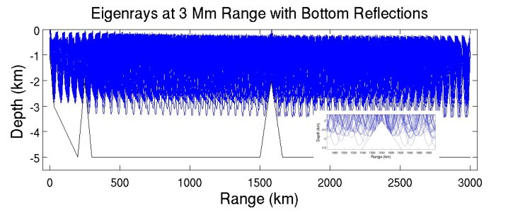
Compute time for eigenray with 4000 rays at 3 Mm range
*aogreef's cpu's have their powersaving mode turned on so that when idle, the cpu frequency is 1 GHz. Such cpu's take a moment to spin up for a process, as a result the benchmark numbers on this lightweight test are a slower than they should be.
Benchmarks (old version)
Compute time for eigenray with 4000 rays at 3 Mm range
Caveats and WarningsThis code is designed for the sole purpose of obtaining rays and travel times for ocean acoustic tomography. It is designed to be as fast as possible in doing that. Hence, it has limitations for other applications. Use the proper tool for the job... The code does not calculate an intensity or other parameters that may be of interest. The Bowlin Ray code makes an estimate of intensity, although the accuracy of such results from rays leaves much to be desired. For intensity, a full-wave calculation, such as from the Parabolic Equation (PE) approach, would be better suited. For really accurate calculations, such as for researching the detailed effects of internal waves on acoustic propagation, the code is probably not suitable, though it could likely give a rough idea of the effects. The problem is that there is a slight numerical "jitter" in the results, so that, when examined under a microscope, the arrivals on the branches of a time front will not be continuous as angle is varied. The code is perfectly suitable for tomography purposes, but not so suitable for this kind of detailed study that demands extraordinary accuracy. For code that will work for those purposes, contact, e.g., Mike Wolfson or John Colosi. The code is dimensioned for ordinary acoustic propagation in the ocean - with sound speed profiles every 100 km or so, say (200 profiles maximum), and less than 100 values of sound speed with depth. In addition, the code relies on sound speed tables that sample sound speed at 3-m intervals over the water column. So attempting to use profiles every kilometer horizontally and every meter vertically is likely to fail. Such situations will require a revision to the code and a recompile...and a revision requiring more than just a change in the dimensions of the arrays, generally.
TODO ListThese are a list of improvements or changes to the code that would be nice to implement someday. If someone should resolve some of these, by all means send the code on to me for implementation!
Copyright © 2008-2015 by the contributing authors. All material on this collaboration platform is the property of the contributing authors. | |||||||||||||||||||||||||||||||||||||||||||||||||||||||||||||||||||||||||||||||||||||||||||||||||||||||||||||||||||||||||||||||||||||||||||||||||||||||||||||||||||||||||||||||||||||||||||||||||||||||||||||||||||||||||||||||||||||||||||||||||||||||||||||||||||||||||||||||||||||||||||||||||||||||