Salinity fluxes in the subtropical gyre
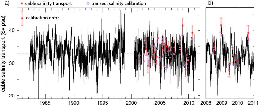
A submarine cable across the Florida Straits has used motionally induced voltages to provide volume transport and temperature transport since 1982 and is an integral part of calculating overturning circulation and heat flux as part of the 26°N overturning array. Here, we calibrated the cable for salinity transport with a new dataset of CTD/LADCP calibration transects. This data set provides volume and temperature transport calibrations that are consistent with earlier measurements. Relative to the basin-averaged salinity (35.156 psu), the Florida Current carries salt northward with a magnitude of 33.0 Sv psu and has a 90th percentile range of 29.1–37.4 Sv psu. The calibration is accurate to 2.2 Sv psu.
With concurrent measurements of velocity, temperature, and salinity, the spatial patterns of variability were investigated to see why a salinity calibration is possible. Despite spatial patterns of salinity variability not overlapping those of velocity, there is still a strong correlation because net volume transport is what drives northward salt transport. Although the same is true for temperature transport, better spatial overlap between temperature and velocity fluctuations leads to a slightly stronger correlation for temperature transport than for salinity transport. Ultimately, it is the high average electrical conductivity and the favorable geometry of the Florida Straits that enables the cable-measured voltage to be accurately calibrated for volume transport. This salinity calibration is a necessary component for closing the freshwater budget at 26°N and for further investigations of subtropical circulation.
Szuts, Z.B. and C. Meinen. 2013. Salinity transport in the Florida Straits. J. Atmos. Ocean. Tech. 5: 971–983. doi: 10.1175/JTECH-D-12-00133.1 author's version (1.5 MB)
Baroclinic waves across a subtropical gyre
A moored array across the Atlantic at 26°N has been used to calculate the overturning circulation since 2004. The mooring data also provide detailed information on low-frequency internal waves. These baroclinic features were examined with a vertical mode decomposition, and by comparison with satellite altimetry. Moorings are located along the eastern boundary off the coast of Africa (EBH), 1200 km offshore (EB1), on the western flank of the Mid-Atlantic Ridge (Marw), and 500, 40, and 15 km from the western boundary at the Bahamas (WB5, WB3, and WB2).
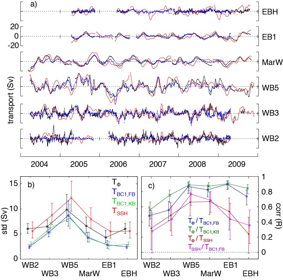
At right are: (a) equivalent volume transports at each mooring calculated from the direct observations (black), from the first-mode reconstruction (blue), and from an SSH reconstruction (red); (b) their standard deviations; and (c) correlations between these quantities. Two different vertical modes are used, classical flat-bottomed (FB) modes, and modes from Killworth and Blundell (KB, 2003).
Away from the boundaries, the vertical structure is almost entirely described (60% variance) by large oscillations of the first baroclinic mode and is coherent with altimetric SSH. Within a Rossby radius of the boundary (45 km), however, the first baroclinic mode has reduced energy, the higher baroclinic modes have a larger relative importance, and altimetric SSH loses coherence with the subsurface fluctuations. These details explain why SSH at the boundary is not sufficient for calculating overturning circulation. The results also suggest the presence of a boundary-trapped annual wave at the eastern boundary.
Szuts, Z.B., J.R. Blundell, M.P. Chidichimo, and J. Marotzke. 2012. A vertical-mode decomposition to investigate low-frequency internal motion across the Atlantic at 26°N. Ocean Sci. 8: 345–367. doi: 10.5194/os-8-345-2012 manuscript (4.2 MB)
Motional Induction
Motional induction is the process that generates electric fields and electric currents in the ocean. The motion of charged ions dissolved in seawater through the Earth's magnetic field acts as a battery that sets up circuits in the ocean. Though very weak (order 1 μV), these signals are measurable and are used by physical oceanographers to calculate water velocity. The circuits formed are almost entirely horizontal, a result of the thin aspect ratio of the ocean (horizontal scales are always much larger than the water depth).In graduate school, I extended motional induction theory to include gradients on short horizontal scales that challenge the 1D assumption of a thin ocean. Such higher order perturbations allow 2D spreading to occur but are hard to calculate exactly. I used analytical, numerical, and observational techniques to quantify the magnitude of such perturbations on velocity calculated from in situ electric measurements.
-
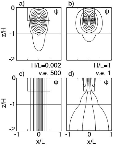
The first source of short scales is narrow velocity features. At right is a schematic of the electromagnetic circuits generated by wide (left) and narrow (right) velocity jets over a stationary deep ocean and a underlying sediment layer, for the electric current stream function \(\psi\) (top, \( \boldsymbol{J} = \nabla \times \psi\)) and the electric potential (bottom, \( \boldsymbol{E} = - \nabla \phi\)). A narrow surface jet enables the electric potential, and thus the electric field, to become vertically non-uniform in the surrounding ocean (z/H < -1) and sediment (-1 ≤ z/H ≤ -2). (Note the difference in vertical exaggeration (v.e.) necessary for showing different aspect ratios H/L). Based on the simplified geometry shown, I used analytical methods to calculate velocity errors resulting from a 1D interpretation of 2D electromagnetic fields over the entire 4-dimensional parameter space. Velocity errors are proportional to the second power of the aspect ratio H/L, with weaker dependence on the other non-dimensional parameters. With an upper bound on aspect ratios derived from fluid dynamical constraints (H/L is ≤0.03 for barotropic flow and ≤0.1 for baroclinic flow), the 1D approximation is in error by less than a few percent.
Szuts, Z.B. 2010a. The relationship between ocean velocity and motionally-induced electrical signals, part 1: in the presence of horizontal velocity gradients. J. Geophys. Res. Oceans. 115: C06003. doi: 10.1029/2009JC006053 manuscript (0.7 MB)
-
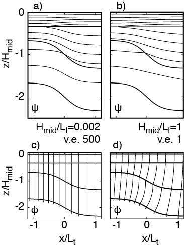
The second source of short scales is steep topography. At right is a schematic of the electromagnetic circuits generated by wide (left) and narrow (right) topographic features in a two-layer ocean with the surface layer in slab motion and with an underlying sediment layer, for the electric current stream function \(\psi\) (top, \( \boldsymbol{J} = \nabla \times \psi\)) and the electric potential (bottom, \( \boldsymbol{E} = - \nabla \phi\)). A steep slope enables the electric field to become vertically non-uniform in the surrounding ocean and sediment. (Note the difference in vertical exaggeration (v.e.) necessary for showing different topographic aspect ratios \(H/L_t\)). Based on the simplified geometry shown, I used a numerical model to calculate velocity errors resulting from a 1D interpretation of 2D electromagnetic fields over the entire 5-dimensional parameter space. As for velocity gradients, velocity errors are proportional to the second power of the topographic aspect ratio \(H/L_t\), with weaker dependence on the other non-dimensional parameters. With an upper bound on topographic aspect ratios derived from observed slope stabilities (typically ≤ 5%, rarely up to 10%), the 1D approximation is in error by less than a few percent.
Szuts, Z.B. 2010b. The relationship between ocean velocity and motionally-induced electrical signals, part 2: in the presence of sloping topography. J. Geophys. Res. Oceans. 115: C06004. doi: 10.1029/2009JC006054 manuscript (1.7 MB)
-
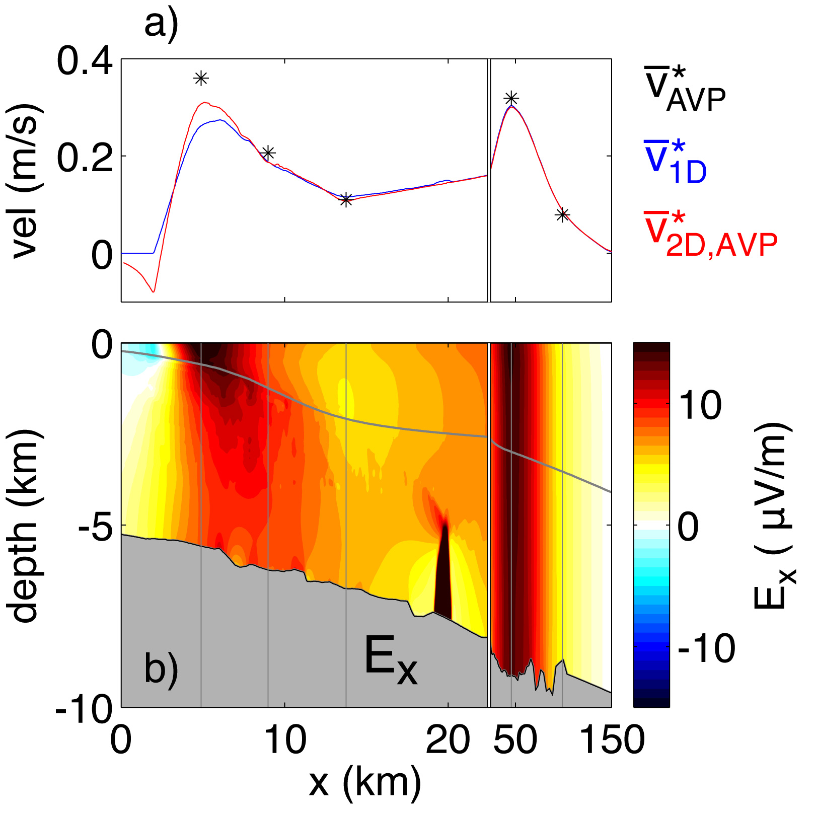
Field observations collected off of Cape Hatteras, a region characterized by a narrow north wall of the Gulf Stream and steep topographic slope (T. Sanford, 1992), enabled the theoretical results above to be tested in the real ocean. An electromagnetic numerical model (Tyler et al, 2004) was used to calculate motionally induced fields incorporating detailed geophysical interpretation of the underlying sediment, which enabled more complete interpretation of the sparse in situ observations. At right is the modeled horizontal electric field (b) in the water column (above the gray line) and in the sediment (below the gray line, roughly 5 km thick). The electric field is proportional to the apparent depth-averaged velocity \(\overline{v}^{\,*}\), which is shown in (a) for the exact 2D interpretation (red), the 1D approximation (blue), and the in situ measurements (black). The 2D interpretation is necessary on the upper continental shelf (5 km < x < 8 km).
If the observations are interpreted with the standard 1D approximation, errors in the vertical profile of horizontal velocity are < 3% (1–3 cm/s) and can be corrected with iterative methods. Errors in the depth-averaged velocity are typically < 2 cm/s (10%). The only exception is on the upper continental shelf where meanders of the Gulf Stream's north wall were not measured: in such extreme regions, the modeling suggests the depth-uniform component \(\overline{v}^{\,*}\) can reach 30%.
The errors from horizontal velocity gradients and from sloping topography combine linearly and agree with the theoretical results from Szuts (2010a) and Szuts (2010b). This article gives observational confirmation that interpreting motionally induced electromagnetic fields with the 1D approximation provides velocities with an accuracy of 1–2 cm/s in almost all regions of the world's oceans.
Szuts, Z.B. 2012. Using motionally-induced electric fields to indirectly measure of oceanic velocity: instrumental and theoretical developments. Prog. Oceanogr. 96: 108-127. doi: 10.1016/j.pocean.2011.11.014 author's version (2.6 MB), or contact me for an electronic reprint