BEE 531 Waves
Instructor: Matthew Bruce / mbruce@uw.edu
University of Washington
Wave propagation and ultrasound physics
- Physical description of wave equation and propagation.
- Propagation in different materials.
- Reflection and refraction.
- Attenuation: absorption and scattering.
Wave propagation and ultrasound physics
- Link: Feynman wave equation
- Foundations of Biomedical Ultrasound by Richard Cobbold.
- Diagnostic Ultrasound by Peter Hoskins. (Chapter 2)
- Diagnostic Ultrasound: Principles and Instruments by F. Kremkau
- Ultrasound Bioinstrumentation by D. Christensen
- Link: Dan Russell waves
- Waves Berkeley Physics Course J. Crawford
How does ultrasound work?
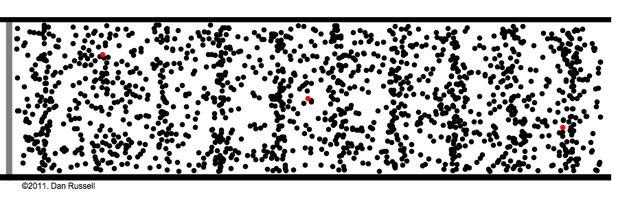
Waves
A collective disturbance in which what happens at any position is adelayed response to the disturbance at adjacent points
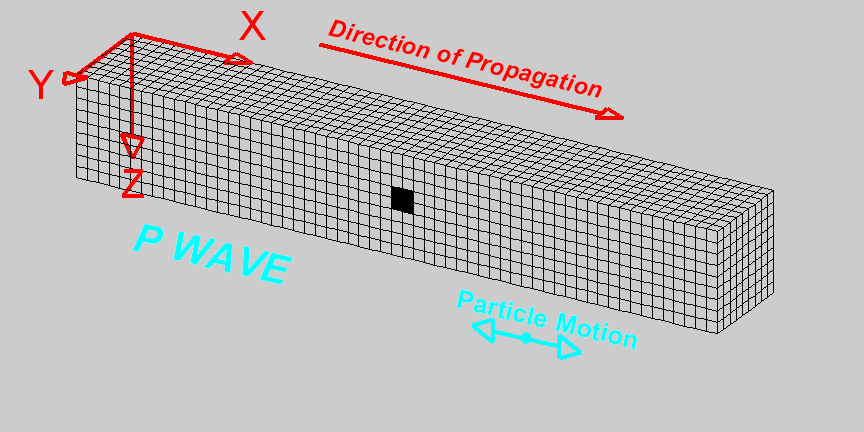
Mechanical waves
Ultrasound
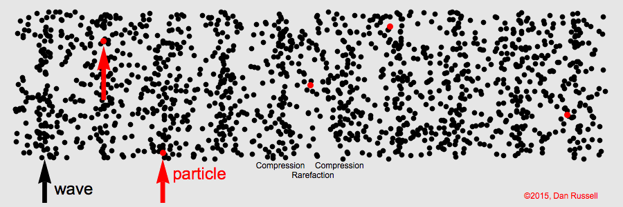
Harmonic traveling wave

wavelength, frequency, wave speed
Pulse wave

Ultrasound
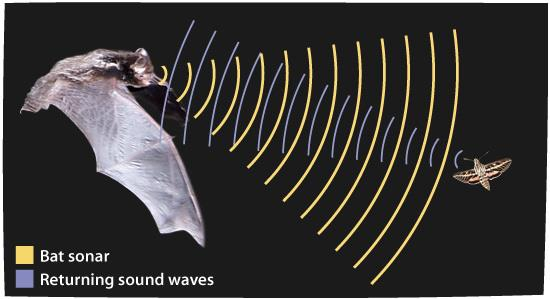
Echo location
Wave equation goals
- How does the wave equation arise?
- Functions of wave equation.
- What determines the speed of sound?
Discretization of the 1D wave equation

Wave equation on a string and discretization

- \( T_1 = T_0 \frac{ y_{i-1} - y_{i} }{\Delta x} \; T_2 = T_0 \frac{ y_{i+1} - y_{i} }{\Delta x} \)
- \( \mu \Delta x \frac{\partial^{2} y_i (x,t)}{\partial t^2} = T_0 \frac{ y_{i-1} - y_{i} + y_{i+1} - y_i }{\Delta x} \)
- \( \frac{\partial^{2} y_i (x,t)}{\partial t^2} = \frac{T_0}{\mu} \frac{ y_{i-1} + y_{i+1} - 2y_i }{\Delta x^2} \)
- \( \frac{\partial^{2} y_i (x,t)}{\partial t^2} = \frac{ y_{i,k+1} + y_{i,k-1} - 2y_{i,k}}{\Delta t^2} \)
- Putting these together: \( \frac{ y_{i,k+1} + y_{i,k-1} - 2y_{i,k}}{\Delta t^2} = \frac{T_0}{\mu} \frac{ y_{i-1,k} + y_{i+1,k} - 2y_{i,k} }{\Delta x^2} \)
- Finally: \( y_{i,k+1} = 2y_{i,k} - y_{i,k-1} \\ + \frac{T_0 \Delta t^2}{\mu \Delta x^2} (y_{i-1,k} + y_{i+1,k} - 2y_{i,k}) \)
- Curvature in x drives the extrapolation of y into the future/next time step.
Extrapolation in the discrete 1D wave equation

- Finally: \( y_{i,k+1} = 2y_{i,k} - y_{i,k-1} \\ + \frac{T_0 \Delta t^2}{\mu \Delta x^2} (y_{i-1,k} + y_{i+1,k} - 2y_{i,k}) \)
- Curvature in x drives the extrapolation of y into the future/next time step.
Step across to fill in space-time grid


Acoustic wave equation assumptions
Assumptions in the following derivation:
- In air \(2.7\times 10^{19} \) molecules in a cubic centimeter vs \(3.3\times 10^{22} \) in water.
- Wavelength is much larger than inter-molecular/atomic spacing (water = 0.3 nm/air = 3.4 nm).
- Ignore the discrete nature of the medium.
- For example 100 GHz wave has a wavelength of 14 nm in water.
- Small changes in pressure/density relative to equilibrium.
Acoustic wave equation derivation
The physics of sound waves involves 3 phenomenon:
- Gas moves and changes density.
- Change in density causes increase in pressure.
- Change in pressure causes gas motion.
3. Change in pressure causes gas motion
Equation of the motion produced by an imbalanced pressure gradient:
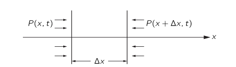
- Thin slab of \( \rho_o \frac{\partial^{2} \chi (x,t))}{\partial t^2} \Delta x \)
- Force on the slab is \( P(x,t)-P(x+ \Delta x,t) = -\frac{\partial P}{\partial x} \Delta x \).
- Putting these together: \( -\frac{\partial P}{\partial x} \Delta x = \rho_o \frac{\partial^{2} \chi (x,t))}{\partial t^2} \Delta x \approx ma \)
2. Increase in density leads to increase in pressure
Small excursion in density leads to small excursion in pressure:
\[
\small{1. \: P = P_o+P_e \quad \rho = \rho_o + \rho_e \\
2. \: P_o+P_e = f(\rho_o + \rho_e ) = f(\rho_o) + \rho_e f^{\prime} (\rho) |_{\rho=\rho_o}\\
3. \: P_e =\rho_e f^{\prime} (\rho) |_{\rho=\rho_o} \\
4. \: P_e =\kappa \rho_e \quad \textrm{where} \; \kappa = f^{\prime} (\rho) |_{\rho=\rho_o} = \frac{\partial P(\rho)}{\partial \rho}|_{\rho=\rho_o}
} \]
1. Gas moves and changes density
Differential displacements in space lead to perturbations in density:
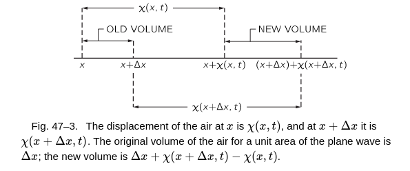
- Thin slab of \( \rho_o \Delta x = \rho ((x+ \Delta x) + \chi (x + \Delta x,t) - (x + \chi (x,t)) \)
- Since, \( \Delta x \) is small: \( \: \chi (x + \Delta x,t) - \chi (x,t) = \frac{\partial \chi(x,t)}{\partial x} \Delta x \)
- Putting these together: \( \: \rho_o \Delta x = \rho (\frac{\partial \chi(x,t)}{\partial x} \Delta x) + \Delta x \)
- Or: \( \: \rho_o = (\rho_o + \rho_e) \frac{\partial \chi(x,t)}{\partial x} + \rho_o + \rho_e \)
- Since \( \rho_e, \: \frac{\partial \chi(x,t)}{\partial x} \) are small: \( \rho_e = -\rho_o \frac{\partial \chi(x,t)}{\partial x} \)
Wave equation derivation
-
Combining 1, 2, 3:
- Gas moves and changes density.
- Change in density causes increase in pressure.
- Change in pressure causes gas motion.
We can sub 2 into 3, \( \rho_o \frac{\partial^{2} \chi (x,t))}{\partial t^2} = \kappa \frac{\partial \rho_e}{\partial x} \).
We can sub 1 into this to remove \( \rho_e \), \( \frac{\partial^{2} \chi (x,t))}{\partial t^2} = \kappa \frac{\partial^2 \chi}{\partial x^2} \) where \( \: c_s = \sqrt{ \kappa} = \sqrt{\frac{dP}{d \rho}} = \sqrt{\frac{P_0}{ \rho_0}} = \sqrt{\frac{K}{\rho}} \).
Traveling waves
Solutions to the wave equation have the following form \( \chi(x,t) = f(x-vt) \) or \( f(x+vt) \).
Lets see if our equation support these solutions:
\[ \scriptsize {1. \frac{\partial^2 \chi(x,t)}{\partial x^2} = f^{\prime \prime} (x-vt) \\ 2. \frac{\partial^2 \chi(x,t)}{\partial t^2} = v^2 f^{\prime \prime} (x-vt) \\ } \]Sinusoidal waves
\( y(x_1,t) = sin(k(x_1-ct)) \) where $k=\frac{2 \pi}{\lambda}$
For a fixed point in space, the sinusoidal wave will oscillate with a period T:
\[ \scriptsize {1.\; kcT = 2 \pi \\ 2. \; \textrm{So, the frequency: } \\ \quad f = \frac{1}{T} = \frac{kc}{2 \pi} = \frac{c}{\lambda} \\ 3. \; \lambda = \frac{c}{f}, \; \textrm{source determines} \; f} \]How does pressure change with density in air?
Newton assumed isothermal changes in pressure/density and got pretty close to the true speed of sound in air.
But over the long wave lengths/time scales air behaves more adiabatically as the rarefaction/compressions pass.
\[ \scriptsize { PV^\gamma = constant \text{, which with density} P = const \: \rho^\gamma \\ \frac{dP}{d \rho} = \frac{\gamma P_0}{\rho_0} \mbox{ which gives for the speed of sound:}\\ \mbox{ Using the ideal gas law, } c_s = \sqrt{\frac{\gamma P_0}{\rho_0}} = \frac{\gamma k T}{m} = \frac{\gamma R T}{\mu} = (\frac{\gamma}{3})^{1/2} v_{avg} } \]Relating temperature to molecular speeds
Newton assumed isothermal changes in pressure/density and got pretty close to the true speed of sound in air.
But over the long wave lengths/time scales air behaves more adiabatically as the rarefaction/compressions pass.
\[ \scriptsize { PV^\gamma = constant \text{, which with density} P = const \: \rho^\gamma \\ \frac{dP}{d \rho} = \frac{\gamma P}{\rho} \mbox{ which gives for the speed of sound:}\\ c_s = \frac{\gamma P}{\rho} = \frac{\gamma k T}{m} = \frac{\gamma R T}{\mu} = (\frac{\gamma}{3})^{1.2} v_{av} \mbox{ using the ideal gas law.} } \]Relating temperature to molecular speeds
Newton assumed isothermal changes in pressure/density and got pretty close to the true speed of sound in air.
But over the long wave lengths/time scales air behaves more adiabatically as the rarefaction/compressions pass.
\[ \scriptsize { PV^\gamma = constant \text{, which with density} P = const \: \rho^\gamma \\ \frac{dP}{d \rho} = \frac{\gamma P}{\rho} \mbox{ which gives for the speed of sound:}\\ c_s = \frac{\gamma P}{\rho} = \frac{\gamma k T}{m} = \frac{\gamma R T}{\mu} = (\frac{\gamma}{3})^{1.2} v_{av} \mbox{ using the ideal gas law.} } \]Further references
For more detail see Feynman's Physics Lectures vol 1 chapter 47
More on the speed of sound for different materials and mediums.
Medium propagation parameters
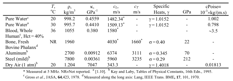
No satisfactory equation of state exists for fluids like we used for air. Measured values of fluid properties are used instead.
Note: Compressibility and Bulk modulus are inversely related.
\( \small{\mbox{Adiabatic Compressibility } \kappa = \frac{1}{V}\frac{\partial V}{\partial p} = \frac{1}{\rho_0}\frac{\partial \rho}{\partial p}} \)Sound propagation in different medium
| Medium | Speed of sound | Wavelength (1 MHz) |
|---|---|---|
| Air | 300 m/s | 0.3x10^6 |
| Water | 1480 m/s | 1.48x10^6 |
| Tissue | 1540 m/s | 1.54x10^6 |
| Bone | 4000 m/s | 4.0x10^6 |
Sound pressure level
Pressure: \( p=\frac{F}{A} \) N/m 2 or Pascals
Atmospheric pressure is 100 kPa, while sound is measured as rms of the deviation from equilibrium:
\[ \scriptsize{ p_{rms} = \sqrt{\frac{1}{t_{avg}} \int_{0}^{t_{avg}} p^2 \,dt } \\ \mbox{for sinusoidal signals of amplitude A, the rms pressure is } A/\sqrt{2} \\ SPL := 20 \log_{10} \left( \frac{p_{rms}}{p_{ref}} \right) } \]- \( p_{ref} = \) 20 µPa threshold of human hearing.
- Ordinary speech: 0.1 Pa SPL = 74 dB
- Close to jet aircraft at take off SPL 120dB
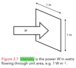
Acoustic Intensity
- Sound transports energy from the source to the medium.
- \( \small{Intensity} = \frac{power}{area}=\frac{work}{area \cdot time} = \frac{force \cdot distance}{ area \cdot time} = pressure \cdot velocity \)
- \( I = pv = \frac{p^2}{Z} = Z v^2 = Watts/m^2.\)
- \( I_{avg} = \frac{1}{t_{avg}} \int_{0}^{t_{avg}} pv \: dt = \frac{p_{rms}^2}{\rho_0 c_0} \) time average
- \( I_{avg} = \frac{p^2}{2 \rho_0 c_0} \) for sinusoidal plane wave
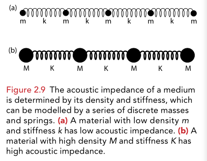
Acoustic impedance
\[ \scriptsize{ Z_0 = \frac{p}{v} = \rho_0 c_0 = \sqrt{K \rho} \\ } \]- where \( \rho_0 \) is the density and \( c_0 \) the speed of sound .
- measure of the reponse of the medium in terms of it's velocity to an applied pressure.
- low acoustic impedance: for an applied pressure, particles are easily displaced.
- high acoustic impedance: for applied pressure, particles resist displacement (density,stiffness).
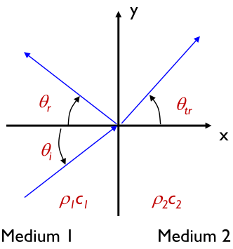
Reflection and transmission
- Reflection coefficient \( R = \frac{p^r}{p^i} \)
- Transmission coefficient \( T = \frac{p^{t}}{p^i} \)
- Two conditions to meet across the boundary:
- Pressure at normal component of velocity must be the same across boundary: \( p^i+ p^r = p^{tr} \; \; \; 1 + R =T \)
Combining the pressure and particle velocity conditions gives:
\( R_p = \frac{Z_2-Z_1}{Z_2+Z_1}, \; \\ T_p = \frac{2Z_2}{Z_2+Z_1}, \; \)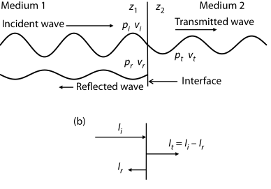
Reflection coefficients for intensity
- For intensity the reflection/transmission coefficients:
- \(I_i = I_t+I_r \)
\( R_I = \frac{I_r}{I_i} =R^2 = \frac{Z_2-Z_1}{Z_2+Z_1} \\ T_I = \frac{I_t}{I_i} = T^2\frac{Z_1}{Z_2} \\ \)
Reflection from a rigid wall
- Rigid wall: infinitely hard medium 2 \( \; \; Z_2 \gg Z_1 \mbox{, } R \approx 1, T \approx 2\)
- Using method of images, pressure at the wall twice incident field. \( \; \; p_{wall} = p^i+p^r = (1+R)p^i = 2p^i \)
- This is called pressure doubling. Notice T=2, even though no energy/particle displacement penetrated into the wall.
Reflection from a pressure release
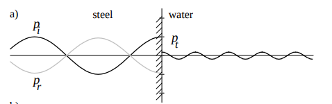
- Infinitely soft medium 2 \( \; \; Z_2 \ll Z_1 \mbox{, } R \approx -1, T \approx 0\)
- Using method of images, pressure at the wall falls to zero. \( \; \; p_{wall} = p^i+p^r = (1+R)p^i = 0 \)
- Examples: water-air, Bone-tissue.
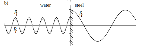
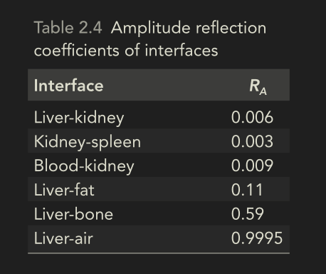
Reflection Coefficients at interfaces
- Impedance similar in soft tissues.
- Even in bone interface, still roughly half the amplitude is coming back
Bounce diagrams
Assume an interface with acoustic impedance\( Z_2= 19 Z_1 \)
\( \; R_p = 0.9 \; \; T_p = 1.9 \)
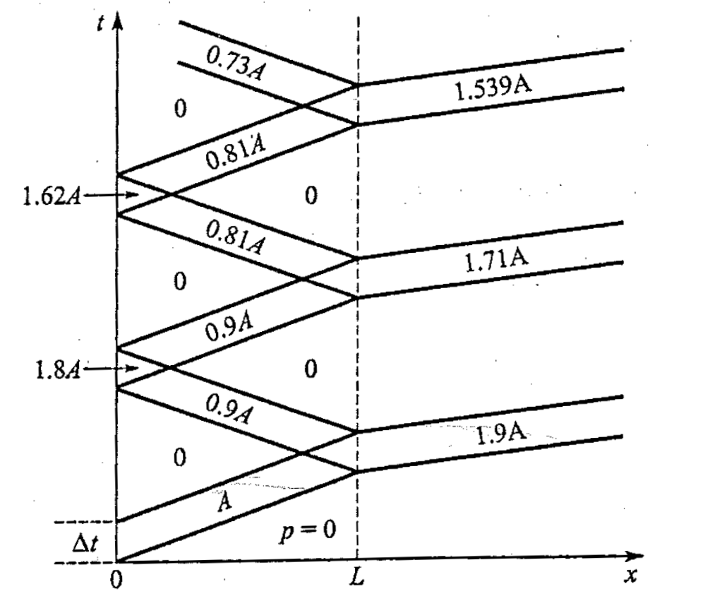
Reflection/transmission is at normal incidence (90 deg) but we plot
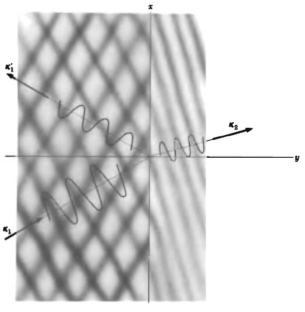
Refraction, Snell's law, oblique incidence
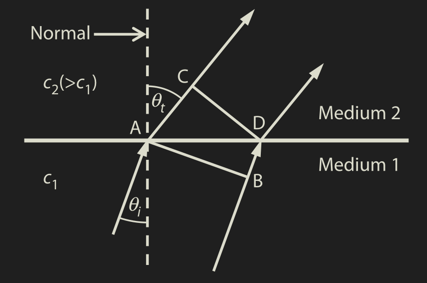
Refraction, Snell's law, oblique incidence
When the angle of incidence is oblique we have the refraction:
\( \; \theta_r = \theta_t, \; \frac{\sin \theta_t}{c_2} = \frac{\sin \theta_i}{c_1} \)The reflection and transmission coefficients then become:
Refraction, Snell's law, oblique incidence
Absorption, scattering and attenuation
- Attenuation of the ultrasound beam is the sum of the scattering and absorption processes \( \; \; \; \; \small{Attenuation = Scattering + Absorption} \)
- Propagation in dissipative fluids
- Physical processes that contribute to dissipation: viscosity (magnitude of internal friction, force per unit area resisting flow), heat conduction, relaxation (restoration of equilibrium following a disturbance)
- Dissipation (thermoviscous) is different from scattering and spherical spreading (strictly a geometrical effect)
- Scattering is the reflection in many directions when the acoustic beam encounters objects that are on the order of a wavelength or smaller
Attenuation power law
- For harmonic plane waves (and here assuming only forwards propagating wave) we can write the acoustic pressure p as
- \( p=Ae^{- \alpha x} e^{j (\omega t - kx)} \;\;\;\;\; I=I_0e^{- 2 \alpha x} e^{j (\omega t - kx)} \)
- Where A is the pressure amplitude at x-0 and \( \alpha \) is the absorption coefficient in nepers per unit distance ("neper" is unitless)
- Very often we use
- \( \alpha_{dB} = 8.68 \alpha \)
- Which has units of dB per unit distance
Review of dB scale
- y in dB -> \( 20 \log_{10} (y) \)
- \( 20 \log_{10} (2) \) \( 20 \log_{10} (10) \)
- Some simple rules with dB
- Powers of 2 -> 6 dB increments
- Powers of 2 -> 6 dB increments
- 2X -> 6 dB increase, 4X -> 12 dB increase
- Powers of 10 -> 20 dB increments
- 10X -> 20 dB increase, 100X -> 40 dB increase
Values of Scattering coefficient in tissue
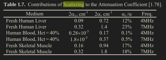
Ref: Cobbold
Specular and speckle
Values of attenuation in tissue
- Attenuation empirically set for different tissues in ultrasound systems.
Values of attenuation in tissue
\( \small{\alpha_{dB} = \alpha[dB/(MHz \cdot cm)] \cdot \Delta x[cm] \cdot f[MHz] = dB }\)
- Attenuation empirically set and estimated for different tissues in ultrasound systems (ref Cobbold).
- Table from Cobbold.
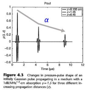
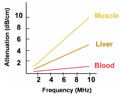
Attenuation frequency dependence
- The frequency dependence of attenuation, α(f) is different in various media depending on their material properties.
- For tissues and fluids, attenuation is related to frequency with a power law
- For Newtonian* fluids it is a quadratic relationship (water, glycerin, castor oil)
- \( \; \; \alpha (f) = \alpha_0 f^\eta \)
- where \( \alpha_0\) is the attenuation coefficient at 1 MHz, f is measured in MHz, and the exponent \( \eta \) is usually between 1 and 2 (Duck 1990; Ophir and Jaeger 1982), depending on the composition and biochemical environment of tissue (Dunn et al. 1969).
- Newtonian fluids: viscous stresses from flow proportional to local strain rate and viscosity tensor does not depend on stress state
Frequency dependence attenuation
\( \small{\alpha_{dB} = \alpha[dB/(MHz \cdot cm)] \cdot \Delta x[cm] \cdot f[MHz] = dB }\)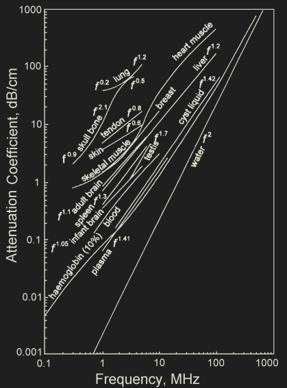
Frequency dependence attenuation
Ref: Cobbold.
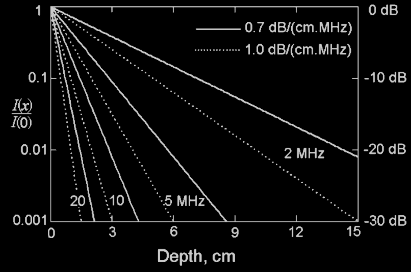
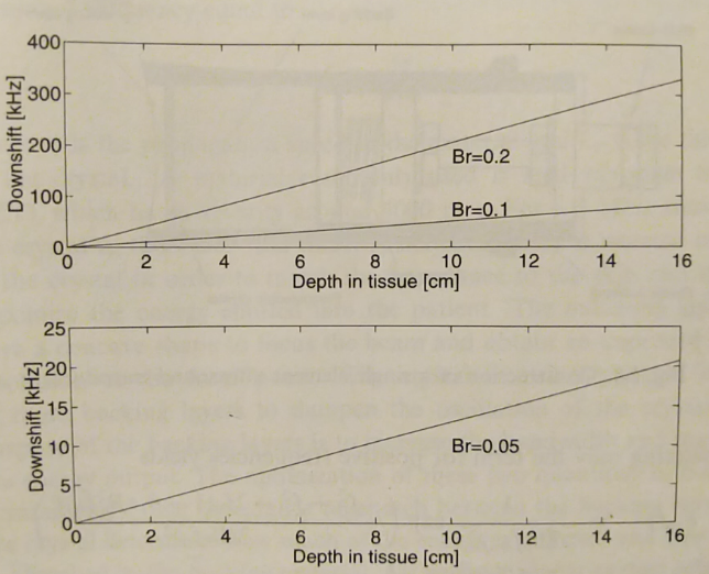
What is the effect of attenuation?
- Attenuation of higher frequencies.
- Results in a linear downshift of center frequency.
- \( \small{p(t)=e^{-2(B_r f_0 \pi)^2 t^2}cos(2 \pi f_0 t) \; \;\;P(f) = \frac{1}{2B_r f_0 \sqrt{2 \pi} }}e^{\frac{-(f-f_0)^2}{2(B_r f_0)^2}} \)
- \( H(f) = e^{ -\alpha_0 f z } \;\;\; P_a(f) = H(f) P(f) \)
- \( f_{mean} = f_0 -(\alpha_0 B_r^2 f_0^2)z \)
3 MHz and 0.5 dB/MHz/cm
Attenuation notes
- Water is considered lossless even in the MHz range. Its thermoviscous absorption is very small and it does not contain any scatterers. (no absorption-no scattering)
- Attenuation is greater in soft tissue, and even greater in muscle. Thus, a thick muscled chest wall will offer a significant obstacle to the transmission of ultrasound. Non- muscle tissue such as fat does not attenuate acoustic energy as much.
- Bone is much more attenuative than muscle and also very reflective (its impedance is much higher than muscle/tissue). Thus it is very hard to image bones.
- Air and lung tissue have very high attenuation and represent severe obstacles to the transmission of acoustic energy.
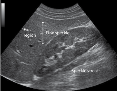
Scattering
- Two principle types in imaging:
- Specular
- Speckle
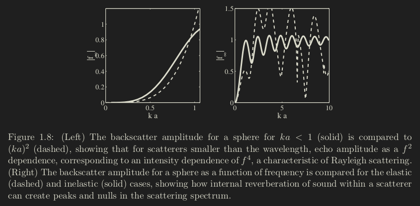
Scattering from sub-wavelength
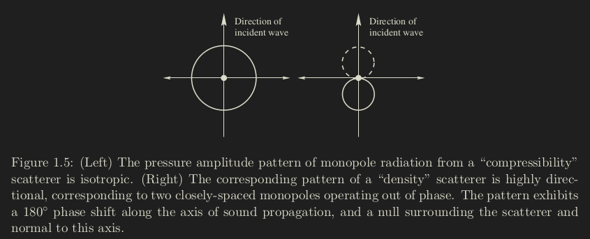
Scattering relative to wavelength
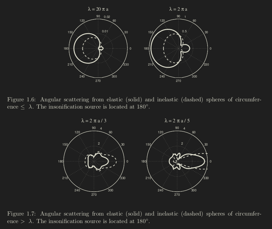
Scattering from sub-wavelength
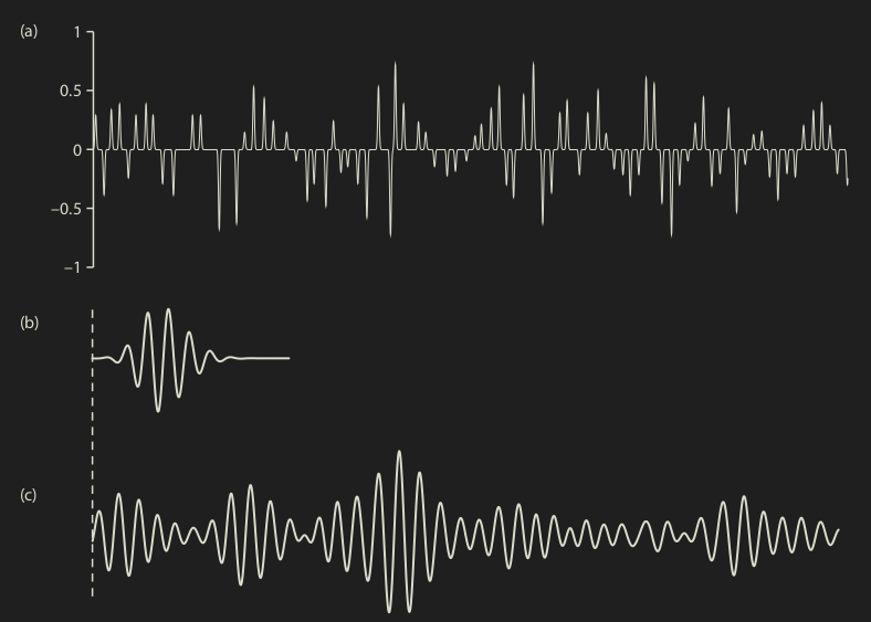
Speckle (multiple scatterers)
Speckle Reduction approaches
- Speckle reduction methods:
- Spatial movement
- Spatial compounding - Angular movement
- Frequency compounding
- Image processing
Spatial compounding
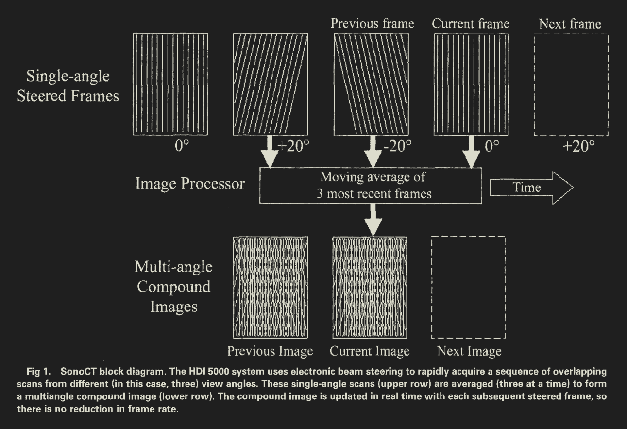
Spatial compounding
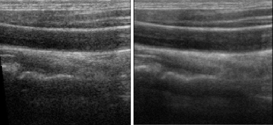
Speckle filtering - no filter
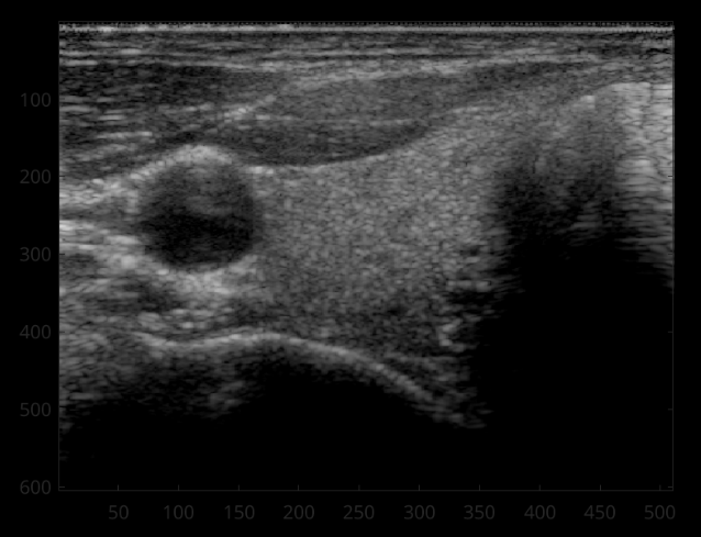
Speckle filtering - filter
