BEE 531 Ultrasound Signal Processing Toolbox
Instructor: Matthew Bruce / mbruce@uw.edu
University of Washington
Signal Processing tools
- Resources
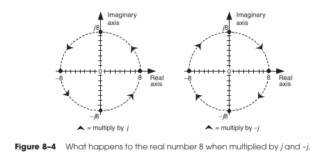
- Complex numbers
- Analytic signals and the Hilbert Transform
- Uses of analytic signals
- IQ approximation
- Discrete Fourier Transform
- Convolution
- Inner workings.
- Filtering
Signal Processing Resources
- Complex numbers: Welch labs
- Link: dsprelated.com
- Understanding digital signal processing by R. Lyons.
- Time Frequency Analysis (Chapter 2) by Leon Cohen.
- The Hilbert Transform by Mathias Johansson
Complex exponential
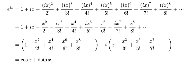
\[ sin(\omega t) = \frac{e^{i \omega t} + e^{-i \omega t}}{2} \]
\[ cos(\omega t) = \frac{e^{i \omega t} - e^{-i \omega t}}{2i} \]
Complex exponential in time
Complex rotation
\[ e^{i \frac{2 \pi k}{N} n} \]
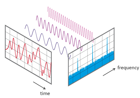
Discrete Fourier Transform
\[ X[k] = \sum_{n=0}^{N-1} x[n] e^{-i \frac{2 \pi k}{N} n} \]
\[ x[n] = \frac{1}{N} \sum_{n=0}^{N-1} X[k] e^{i \frac{2 \pi k}{N} n} \]
Decompose time series into weighted frequency vectors.
YouTube video illustrating this idea. Link
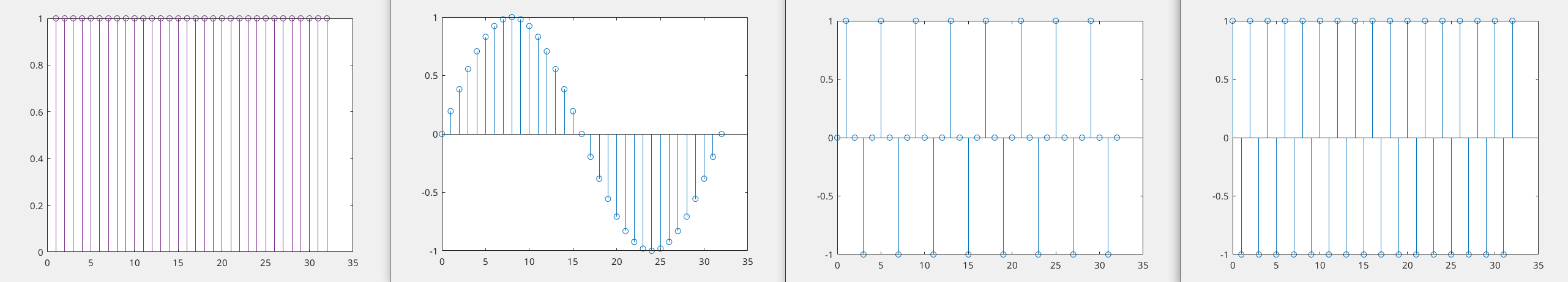
Fourier Vectors
Fourier transform for cont/discrete time/frequency Link
Different forms of Fourier Transform
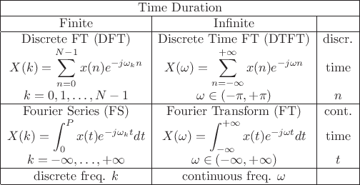
Fourier transform for cont/discrete time/frequency Link
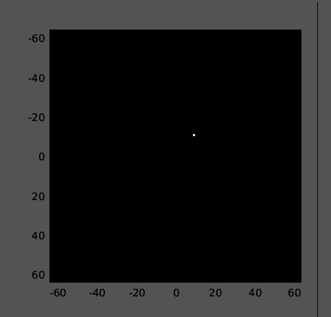
Discrete Fourier Transform
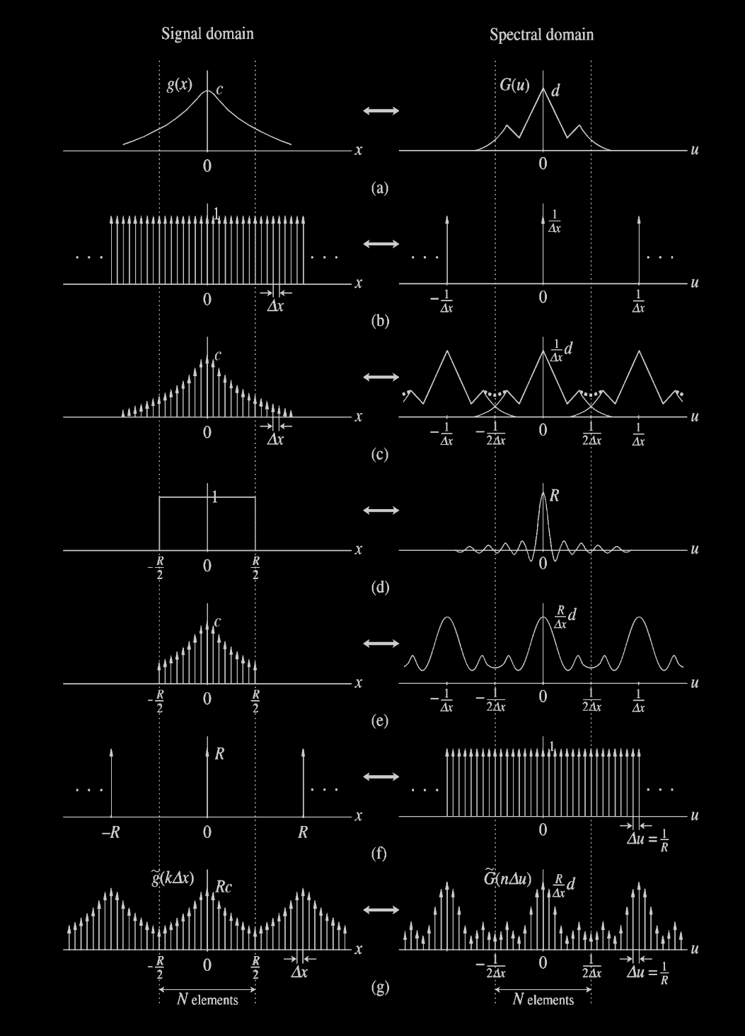
Discrete Fourier Transform
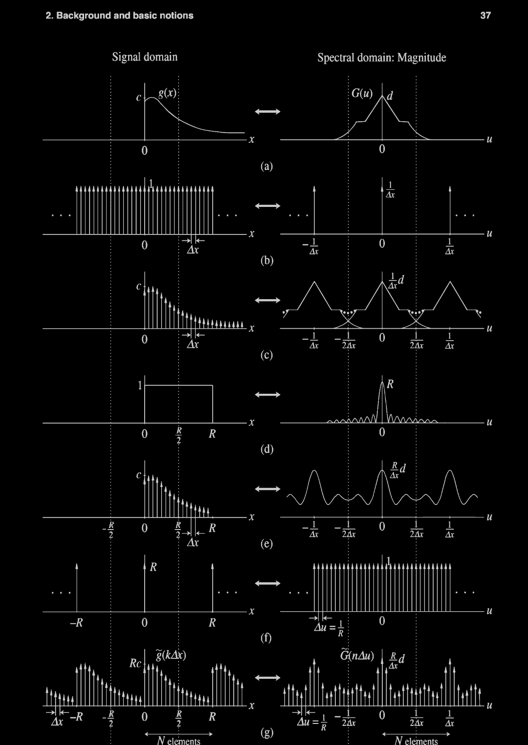
Results in repeated spectra and waveform.Link
Alialsing and DFT
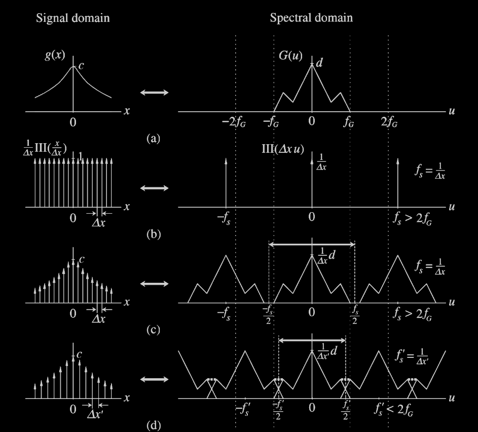
Results in repeated spectra and waveform.Link
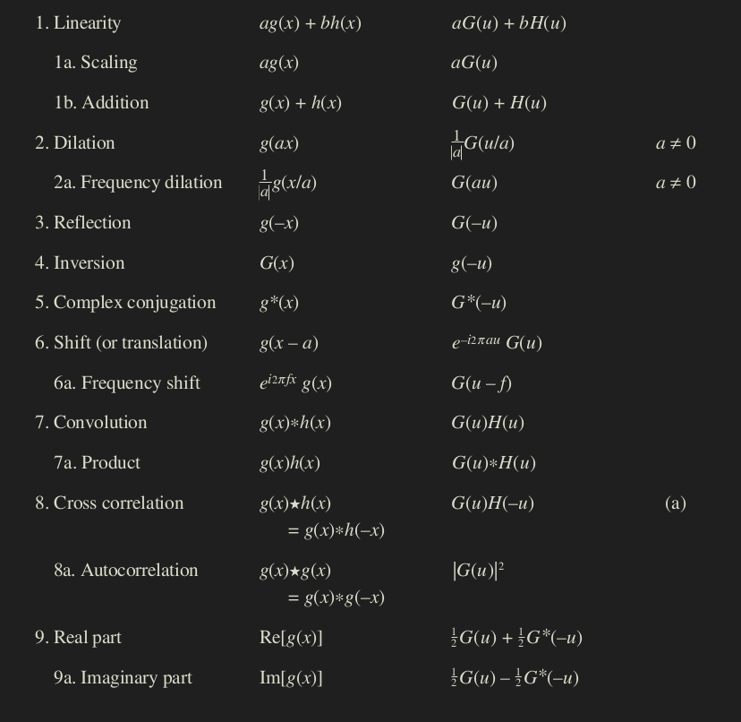
Fourier Transform properties
Results in repeated spectra and waveform.Link
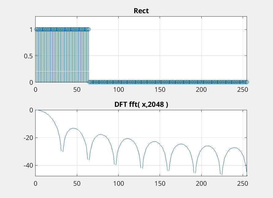
DFT rect
\[ X[k] = \sum_{n=0}^{N-1} x[n] e^{-i \frac{2 \pi k}{N} n} \]
\[ X[k] = \frac{1}{N_0} \frac{\sin ((\pi k L/N_0))}{\sin(\pi k/N_0)} \]
\[ \textrm{where } L=2N + 1 \]
$N_0=2048 \: and \; N = 64$
YouTube video illustrating this idea. Link
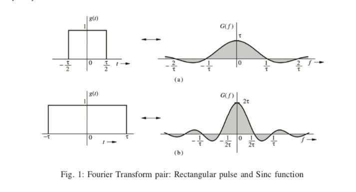
Fourier Transform pairs
Fourier transform link.Link
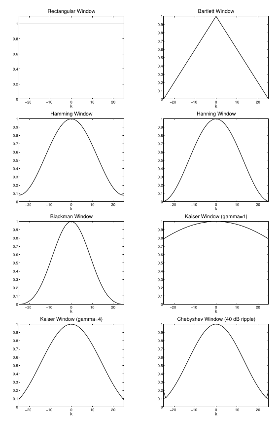
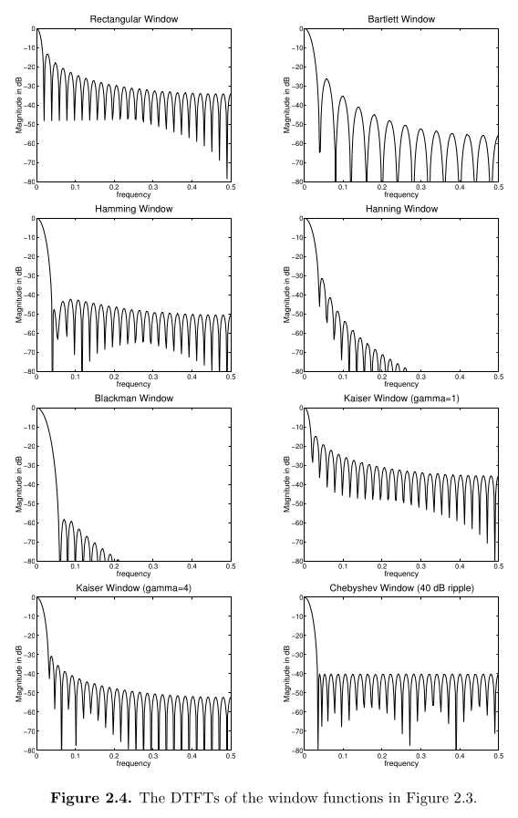
Spectral Analysis and windows
Time bandwidth product
Inverse relationship of pulse duration and bandwidth:
\[ N_e \beta_e = 1 \]
Two dimensional Fourier transform
\[ X[k,j] = \sum_{m=0}^{N-1} \sum_{n=0}^{N-1} x[n,m] e^{-i \frac{2 \pi k}{N} n} e^{-i \frac{2 \pi j}{N} n} \]

YouTube video illustrating this idea. Link
Convolution
- Linear time invariant systems.
- The summation of the trailing impulse responses of the current and previous inputs.
- First order model of a lot of systems.
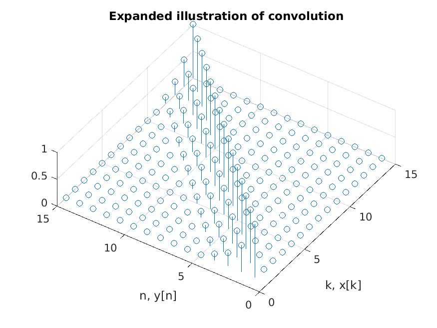
Convolution
\[ y[n] = \sum_{n=1}^{\infty} x[k] h[k-n] \]
The summation of the trailing impulse responses of the current and previous inputs.
\[ Y[k] = H[k]*X[k] \]
YouTube video illustrating this idea. Link
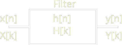
Filter
\[ y[n] = \sum_{n=1}^{\infty} x[k] h[k-n] \]
The summation of the trailing impulse responses of the current and previous inputs.
\[ Y[k] = H[k]*X[k] \]
YouTube video illustrating this idea. Link
Analytic Signals
- It is a convenient representation of real signals (eg harmonic) with useful properties not found in real signals.
- For harmonic signals:
- Enables calculation of instantaneous amplitude.
- Enables calculation of instantaneous phase.
- Simplifies some processing and analysis (e.g. mixing).
- Non sysmetric Fourier spectrum.
- Enables calculation of direction in Doppler processing.
- Can be used advantageously in ultrasound system architectures.
-
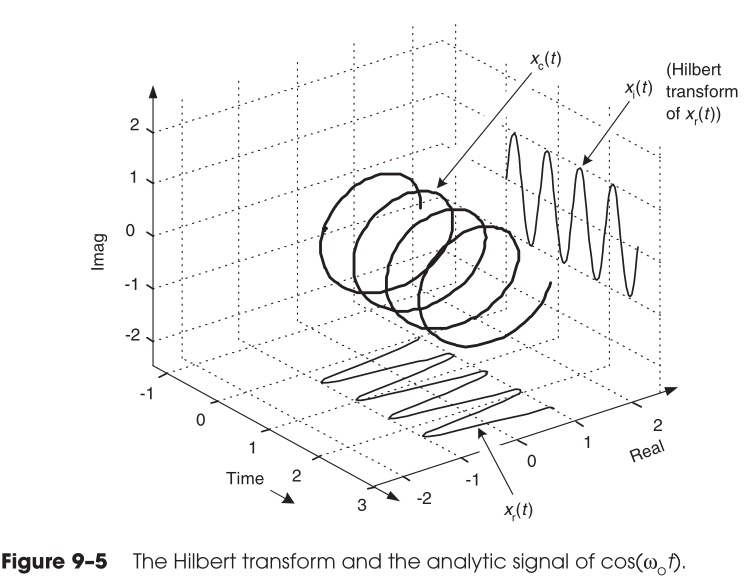
What is an Analytic signal?
- Complex signal with following definition:
- Summation of the real signal plus an imaginary part times the hilbert transform.
- \( z(t) = \color{yellow}{x(t)} + i\color{magenta}{H(x(t))}= A(t)e^{\phi(t)}. \)
- Instantaneous amplitude: \( A(t) = \sqrt{\color{yellow}{x(t)}^2 + \color{magenta}{H(x(t))}^2} \).
- Instantaneous phase: \( \quad \phi(t) = \arctan( \frac{\color{magenta}{H(x(t))}}{\color{yellow}{x(t)}}) ) \).
- Instantaneous frequency: \( \omega(t) = \frac{d \phi(t) }{dt} \).
Hilbert transform introduction. Link
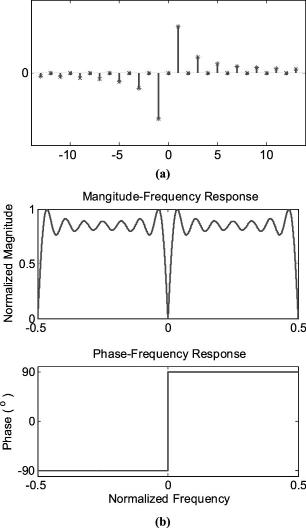
What is an the Hilbert transform?
- Unlike the Fourier transform, the domains stay the same.
- Time domain impulse response:
- \( h(t) = \frac{1}{\pi t}\).
- \( A(r(t)) = x(t) + \frac{j}{\pi} \int_{\infty}^{\infty} \frac{x(\tau)}{t-\tau} d\tau \)
- Frequency domain:
- \( H(f) = jsgn(f) = \begin{cases} -j \; \text{if} \; f>0 \\ 0 \; \text{if} \; f=0\\ j \; \text{if} \; f<0 \end{cases} \)
- \( A(X(f)) = X(f) + H(f)X(f) = 2X(f) \; f>0 \).
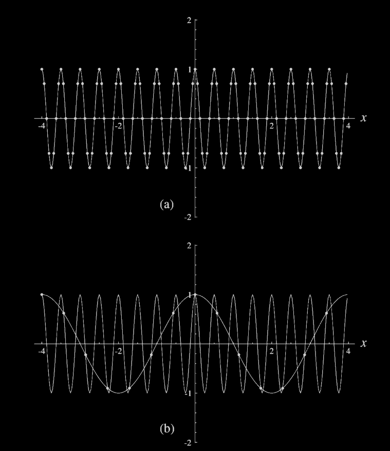
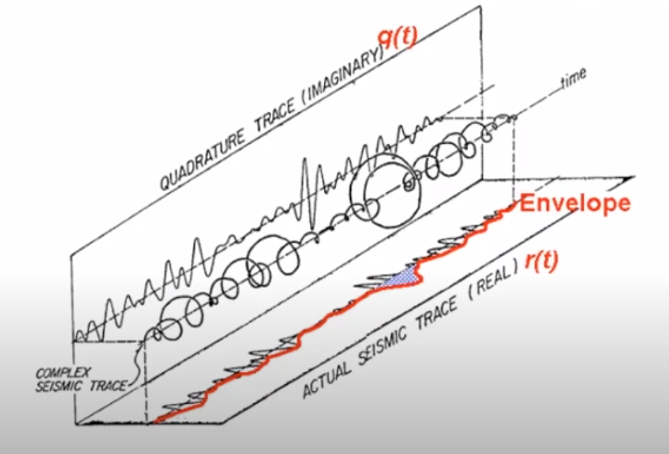
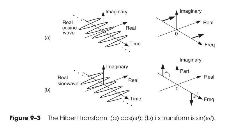
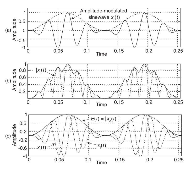
Hilbert transform of a sinusoid
Instantaneous Amplitude
\[ e(t) = \sqrt{ x(t)^2+(H(x(t))^2 } \]
The amplitude of our real waveform is referred to as envelope.
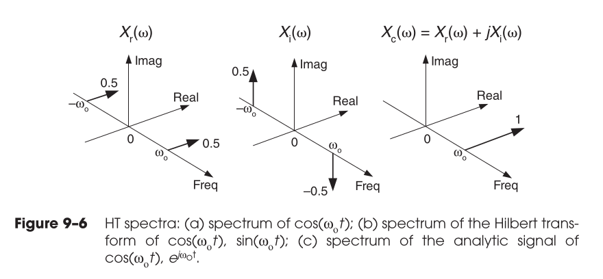
Connection between 90 deg phase shift and cancellation of negative frequencies
\[ x(n) = \sum X(k) e ^{i 2 \pi k/N n} + X(-k) e ^{-i 2 \pi k/N n} \] where $X(k)=X(-k)$ for real signal x(n)
For a real signal, the negative frequency Fourier coefficients serve to zero out the imaginary component of the inverse Fourier transform in order reconstruct the original real signal.
So, if we drop the negative frequencies, we are left with the forward rotating frequencies and a complex signal with a complex component having a 90 deg phase shift.
\[ x(n)+i\color{magenta}{H(}x(n)\color{magenta}) = \sum X(k) e ^{i 2 \pi k/N n} = \sum X(k) cos( 2 \pi k/N n) + i \color{magenta}{ X(k) sin( 2 \pi k/N n)} \]
\[ z(n) = x(n)+i\color{magenta}{H(}x(n)\color{magenta}) \quad FT \quad Z(k) = X(k) + sgn(k) X(k) \quad where \; Z(k) =0 \lt 0 \]
Utility of Analytic Signal
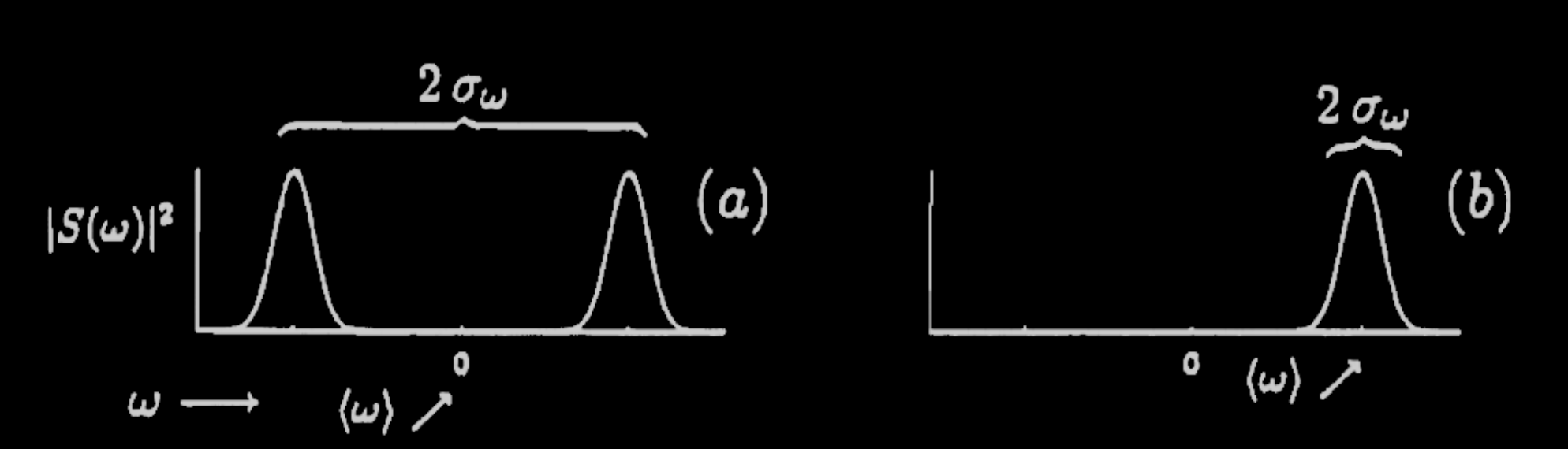
- Real signals have symmetric Fourier transform and zero spectral moments.
- Analytic signals have mean frequency and bandwidts which reflect the spectral content.
What is IQ or quadrature signal?
- It is an approximation to an analytic signal at a signal frequency.
- It is a good approximation when narrowband.
- A measure how good is how much spillage outside of frequencies [0 to in].
- See chapter 8 Understanding Digital Signal Processing by Richard Lyons.
What is IQ or quadrature signal?
Quadrature signal in seismic signal processing
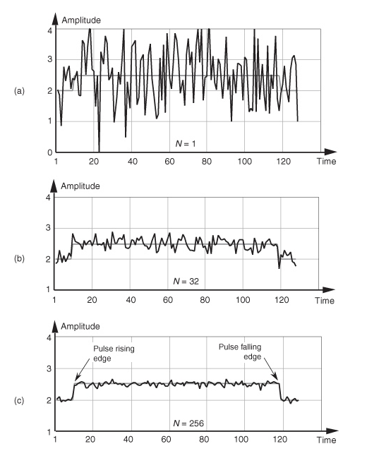
Coherent and incoherent averaging
- Coherent averaging
- Requires the time/phase be the same for each measurement
- \(SNR_{gain} = \frac{SNR_{avg}}{SNR_{in}} = \frac{A/\sigma_{avg}}{A/\sigma_{in}} = \\ \frac{\sigma_{in}}{\sigma_{avg}} = \frac{\sigma_{in}}{\sigma_{in}/\sqrt{N}} = \sqrt{N} \)
- \(SNR_{gain (dB)} = 10 \log_{10}{N} \)
- Incoherent averaging
- No time considerations are made for each measurement
- \(SNR_{dB} = 10 \log_{10}{\sqrt{N}} \)