BEE 531 Ultrasound beams

Why do we care about controlling where our ultrasound goes?

1. Determines our lateral resolution.
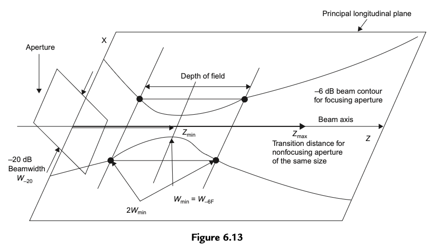
2. Determines depth of field.
3. Reducing off-axis artifacts.
4. Reduces reverberation artifacts.

Foundation of transmit and receive components of ultrasound imaging.

Ultrasound Image artifacts.Ultrasound artifacts

Sound Beams

1. In ultrasound beams are used to guide waves to interact with our medium.
2. A sound beam is bounded in 2 dimensions (x,y) and propagates in a third (z).

Diffraction

• Diffraction is how waves spread around a edge pass through an aperture.
• The abrupt edge of a radiation source like the edge of a piston.
• For arrays, diffraction describes how the sampling of the aperture affects the beam.
• Involves constructive and destructive interference of waves generated at the boundary of the source/obstacle.
• Scattering is typically refered to as diffraction of objects on the order and less than a wavelength.

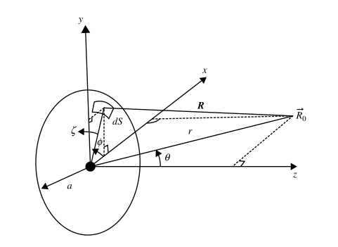
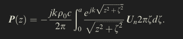
Point Source

\( \nabla^2 p = \frac{1}{c^2} \frac{\partial (p)}{\partial t^2} \\ \) \( \frac{\partial (rp)}{\partial r^2} = \frac{1}{c^2} \frac{\partial (rp)}{\partial t^2} \\ \) \( rp(r,t) = A e^{j(\omega t - kr)} \\ \) \( p(r,t) = \frac{A}{r} e^{j(\omega t - kr)} \)

Point source/wave eq solved in spherical coord's. Link

Superposition/Interference

Two propagating waves results in

\( f_1(x-ct) , f_2(x-vt) \\ \) \( \frac{\partial (f(x,t))}{\partial x^2} = \frac{1}{c^2} \frac{\partial (f(x,t))}{\partial t^2} \\ \) \( f_3(x-ct) = f_1(x-ct) + f_2(x-vt) \)

results in the sum of the two waves.

Simplified wave equations

Propagation in a homogeneous medium with compressibility \( \kappa \), shear and bulk viscosity \( \mu , \mu_B \), \( \mathbf{v}(\mathbf{r},t) = \nabla \phi(\mathbf{r},t) \):

1. Small amplitude compressional wave.
2. \( \mu = \mu_B = 0 \quad (\textrm{no shear and bulk viscosity})\).
3. \( c_0 = \frac{1}{\sqrt{\kappa \rho_0}}= \sqrt{\frac{B}{\rho_0}} \).
4. \( v = - \nabla \phi, \; p= \rho \frac{\partial \phi}{ \partial t} \).

Solving the wave equation

1. Analytic approaches
1. Limited to simple scenarios.
2. Solving Greens function for geometry.
3. Eg. piston, rectangular sources.


2. Numerical approaches
1. Most often used (FEM, FD, angular spectrum).
2. Eg. Fields II, k-wave, MUST, Focus, ...
3. Large numerical packages: Comsol, etc..

Simplified analytic wave solutions

1. Solve Greens function/impulse response.
2. Geometry is flat source into free space.
3. Sometimes leading to Rayleigh integral.
4. Time and frequency domain approaches.
5. eq. (2) sum of point sources over source surface.

Analytic wave solutions

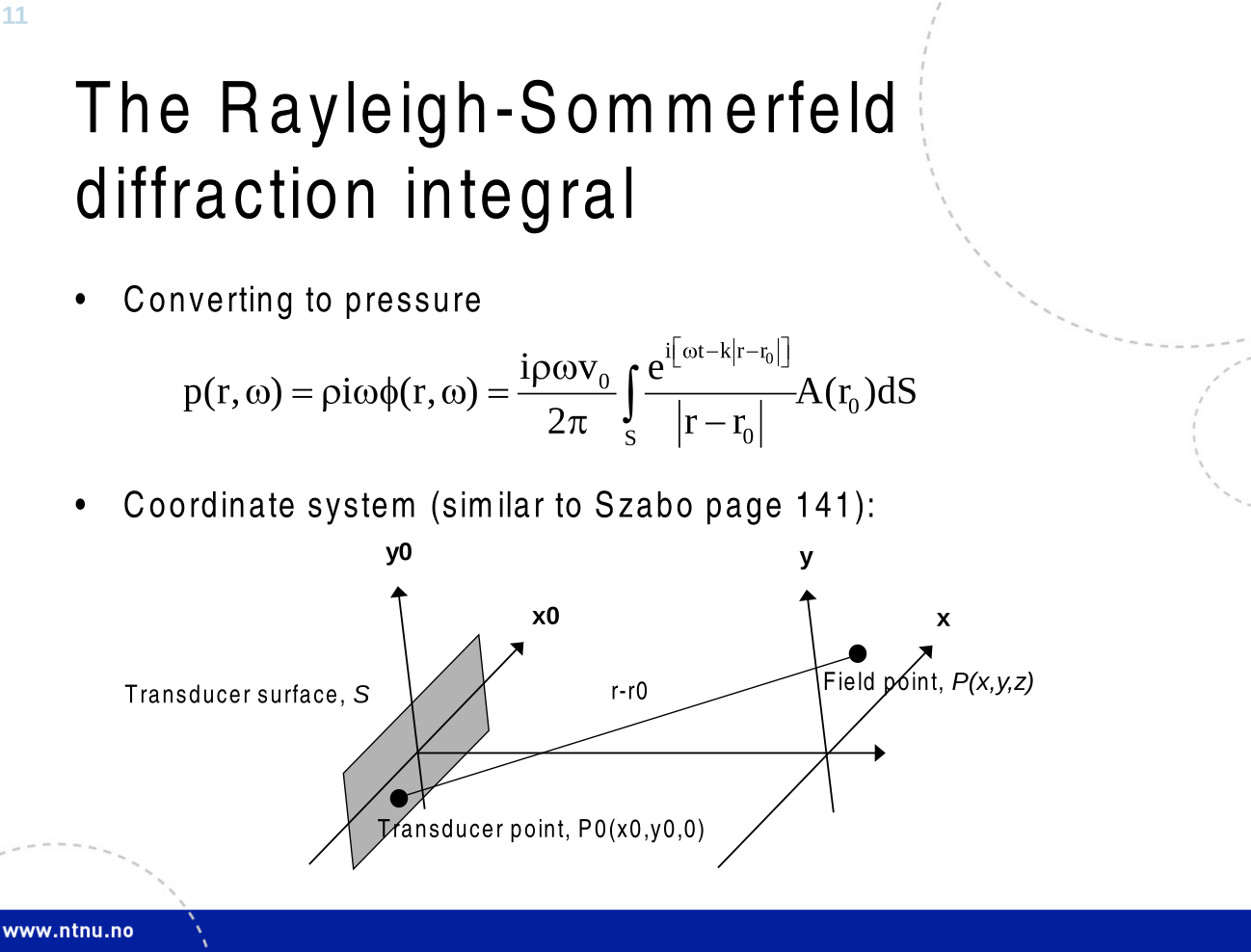
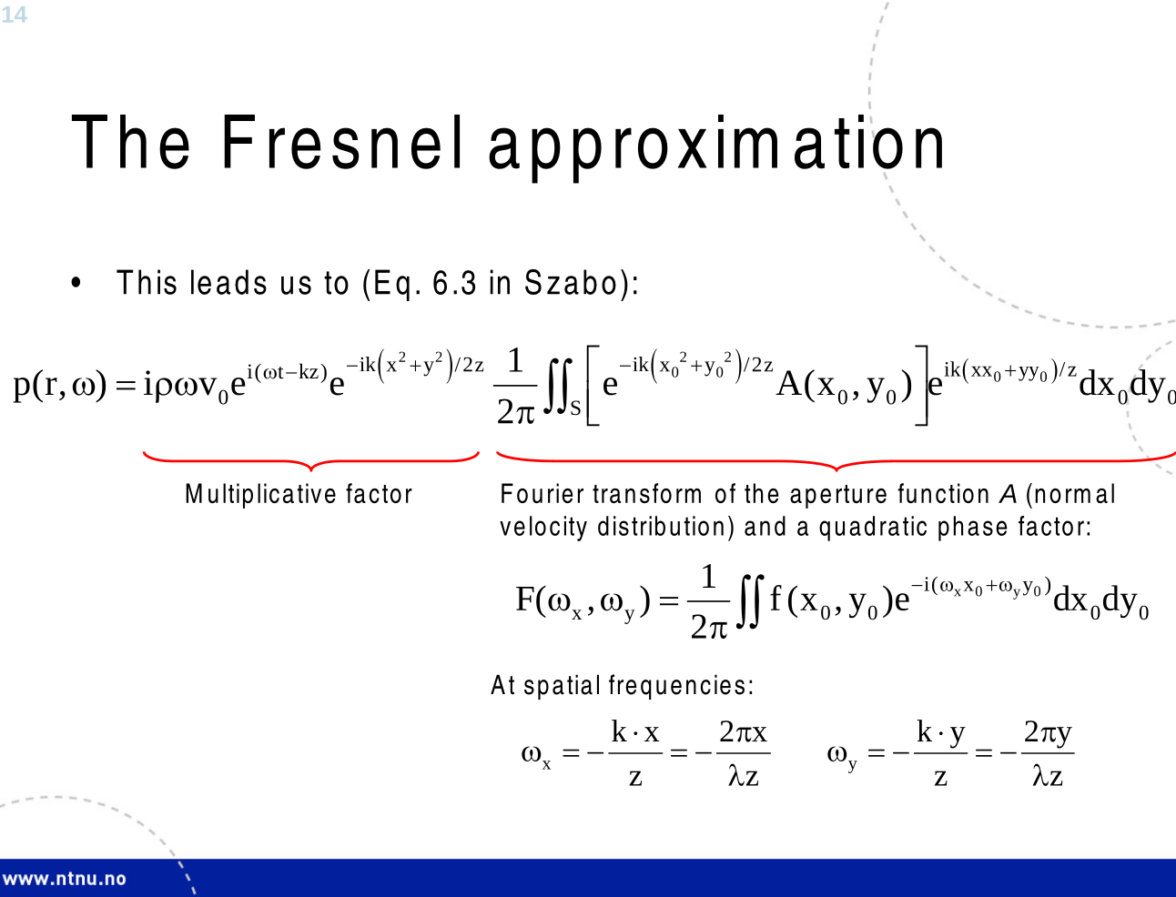
Rayleigh-Sommerfeld diffraction equations:

1. All of the assumptions above plus:
2. Geometry is flat source into free space.
3. eq. (1) For a single frequency sum of point sources over source surface.
4. eq. (2) Time domain point sources over source surface.

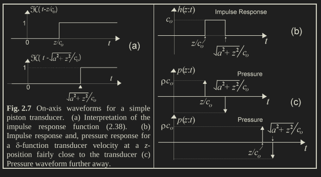
The Rayleigh Integral

Can be expressed as convolution (\( v_n(x,y,0,t)=A(x,y)v_n(t)\)): \[ \phi(\mathbf{r}, t) = \frac{1}{2 \pi} \iint\limits_{S_0} \frac{v_n(t-\frac{R}{c})A(x_0,y_0))}{R} dS_0 \; (2) \quad v_n(t-\frac{R}{c}) = \int\limits_{\infty}^{-\infty} v_n(\tau) \delta(t-\frac{R}{c}-\tau) d\tau \] \[ \phi(\mathbf{r}, t) = \int\limits_{\infty}^{-\infty} v_n(\tau) \color{orange}{\iint\limits_{S_0} \frac{A(x_0,y_0) \delta(t-\frac{R}{c}-\tau))}{R} dS_0}d\tau \]

1. \( \phi(\mathbf{r}, t)=v_n(t) \ast \color{orange}{h(r,t)} \)
2. \( v = - \nabla \phi, \; p= \rho \frac{\partial \phi}{ \partial t} \).
3. \( p(r,t)= \rho v_n(t) \ast \frac{\partial h(r,t)}{ \partial t} \).
4. \( v(r,t) = -v_n(t) \ast \nabla \color{orange}{h(r,t)} \).

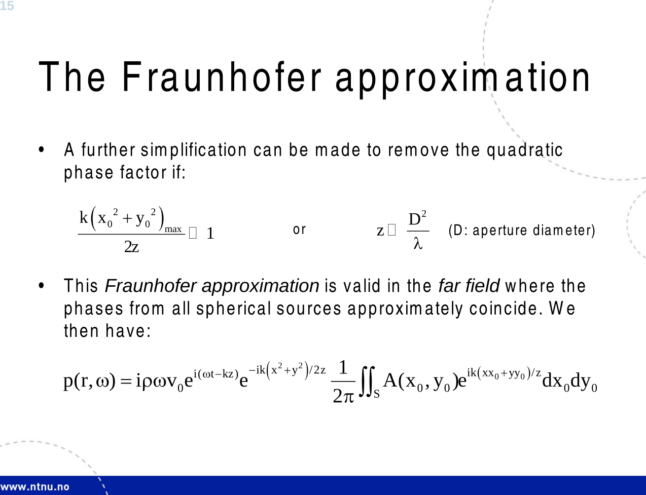
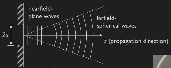
Unfocused piston

\( \nabla^2 P - \frac{\partial P}{\partial t^2} = f(\mathbf{r},t) \\ \)

\( P(\mathbf{r}) = - \frac{jk \rho_0 c}{2 \pi }\int\limits_{S_0} \frac{e^{-jkR}}{R} U_n \, dS_0 \; \\ \)

\( P(r,\theta) = - jk \rho_0 c U_n \frac{e^{jkr}}{r} a^2 \frac{J_1(ka sin \theta)}{ka sin \theta } \\ \)

Unfocused piston: on axis

Sourse: Foundations in Biomedial Ultrasound by Cobbold

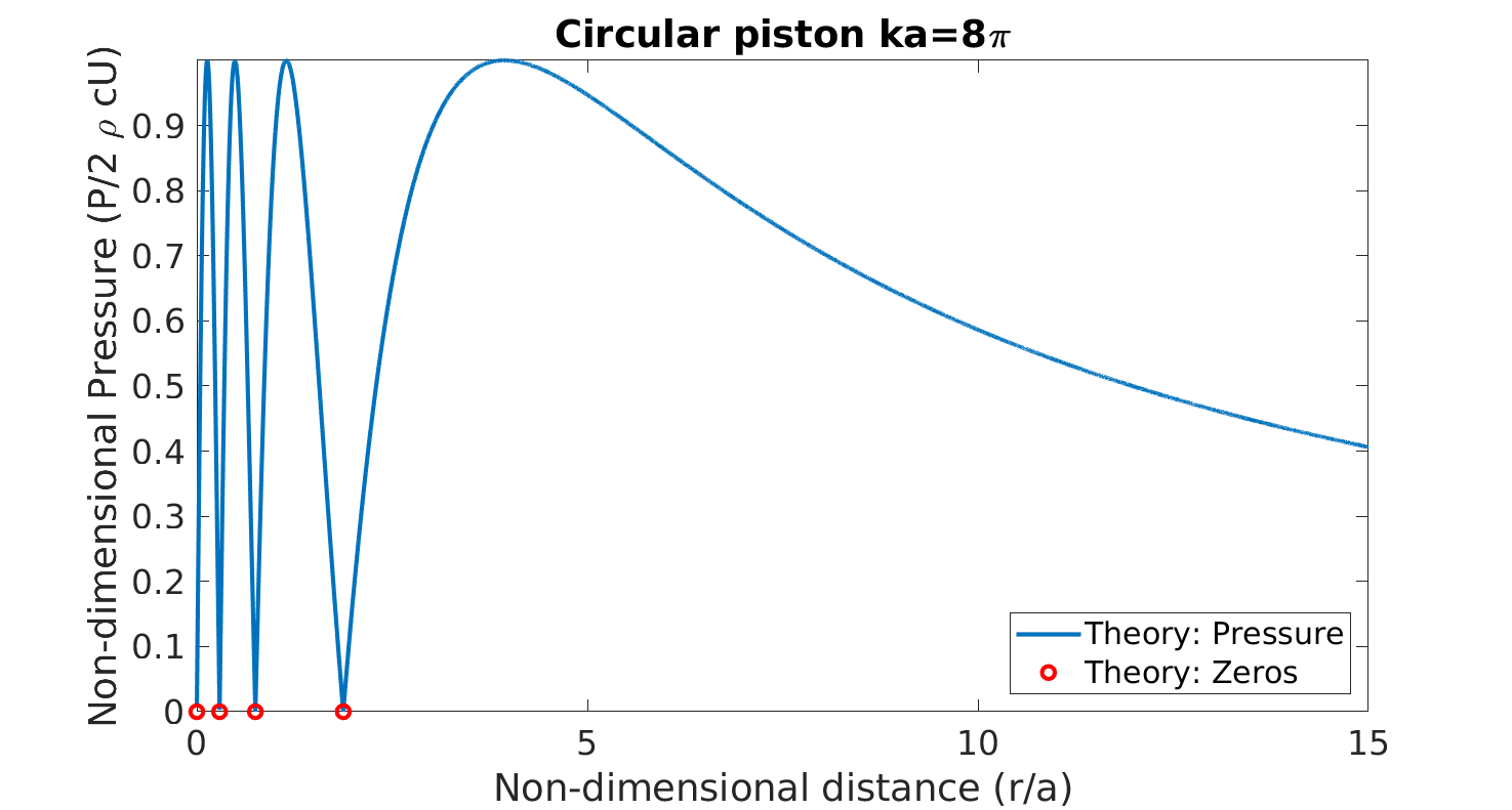
Unfocused piston: on axis

\( P(z,0) = \rho_0 c U_0 (e^{jkz} - e^{jk \sqrt{z^2 + a^2}}) \)

\( P(z,0) = \rho_0 c U_0 (1 - e^{-j k ( \sqrt{z^2 + a^2}-z)} ) \)

\( P(z,0) = 2 \rho_0 c U_0 (sin( \frac{kz}{2} [\sqrt{1 + (\frac{a}{z})^2 } - 1])) \\ \)

If z>>a then the magnitude of field looks like from a point source:

\( P(z,0) \approx 2 \rho_0 c U_0 sin( \frac{ka}{4} \frac{a}{z} ) \approx \frac{1}{2} \rho_0 c U_n ka \frac{a}{z} \\ \)

Unfocused piston: transverse field

\( P(r,\theta) = - jk \rho_0 c U_n \frac{e^{jkr}}{r} a^2 \frac{J_1(ka sin \theta)}{ka sin \theta } \\ \)

\( P(r,0) = - j \rho_0 c \frac{k a^2}{r} e^{jkr} \frac{U_n}{2 } \\ \)

\( P(r,\theta) = P(r,\theta) 2 \frac{J_1(ka sin \theta)}{ka sin \theta } \\ \)

refs: Kinsler-Fund Acoustic waves and Kim-Sound Prop Imp

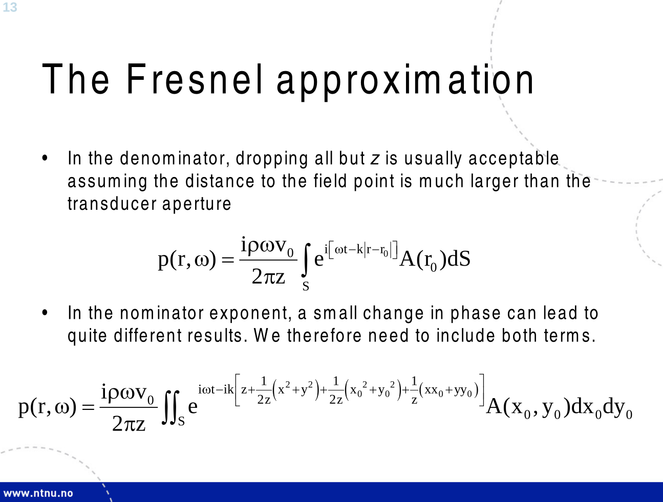
Simple numerical solution to Rayleigh-Sommerfeld equation

\[ p(\mathbf{r}, \omega) = \frac{i\rho \omega v_o}{2 \pi} \iint\limits_{S_0} \frac{e^{-jkR}}{R} A(x_0,y_0) \, dS_0 \]

                 for m=1:100
                    for l=1:100
                       pt(l,m)=0;
                       psum=0;
                       for nrad=1:36
                          sgma=nrad*a/36;
                             for nang=1:36
                                psi=nang*2*pi/36;
                 						    zs=sgma*cos(psi);
                 						    ys=sgma*sin(psi);
                 						    rp=sqrt((zs)^2+(y(l)-ys)^2+x(m)^2);
                 						    dp=exp(-i*k*rp)/rp*sgma;
                 						    psum=psum+dp;
                 				     end
                 		   end
                 		   pt(l,m)=psum;
                 	 end
                 end

           

Homework 2, problem 3: Purdue ME 513 Engineering Acoustics. Link

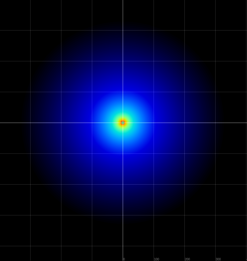
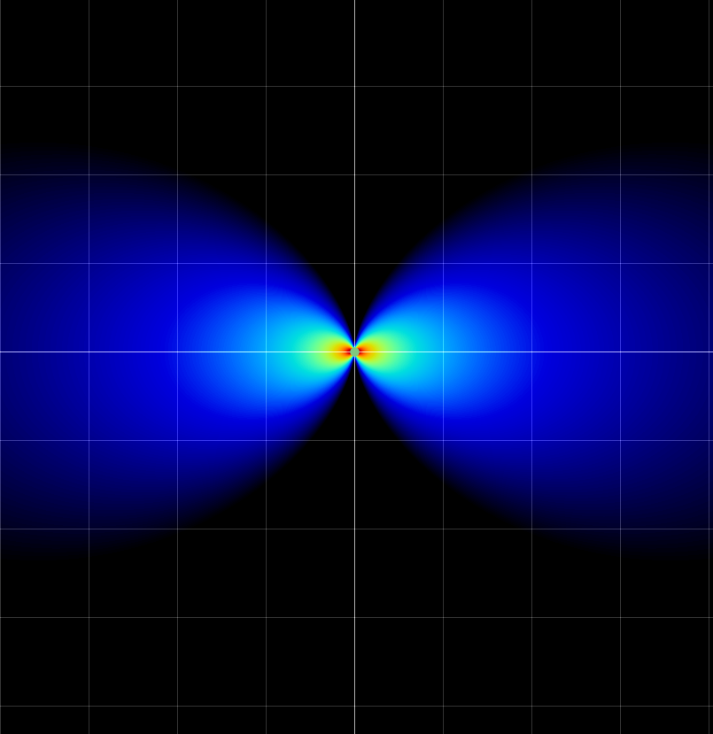
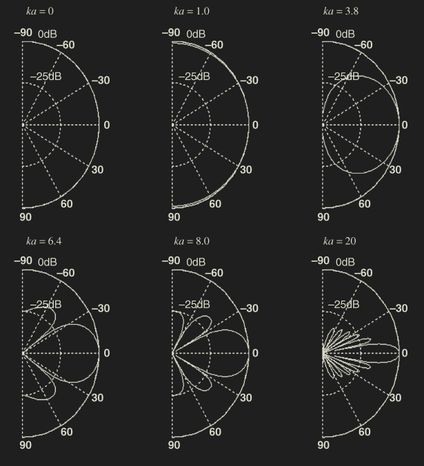
Piston increasing ka

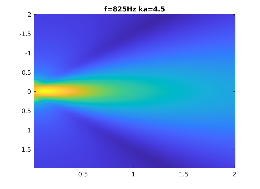
Numerical calculation of Rayleigh integral.

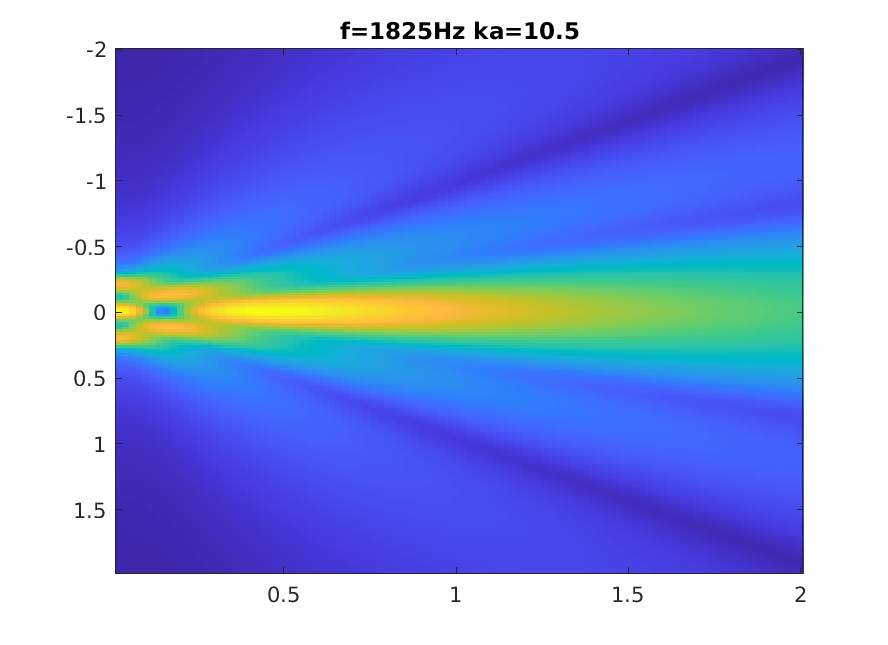
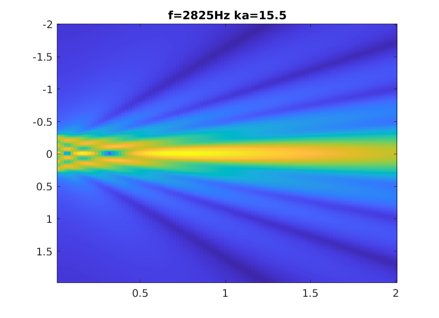
Piston increasing ka

Numerical calculation of Rayleigh integral.

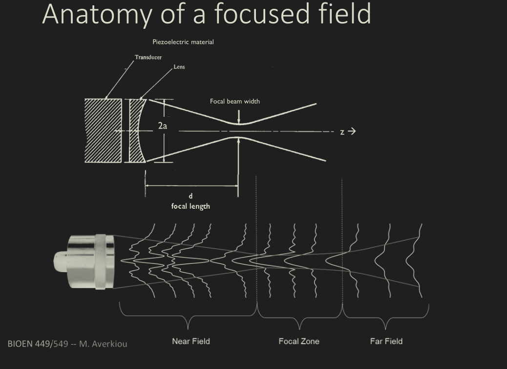
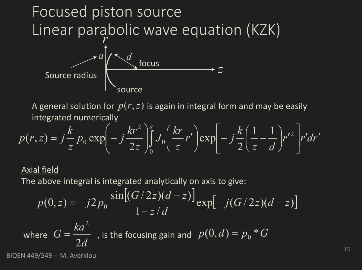
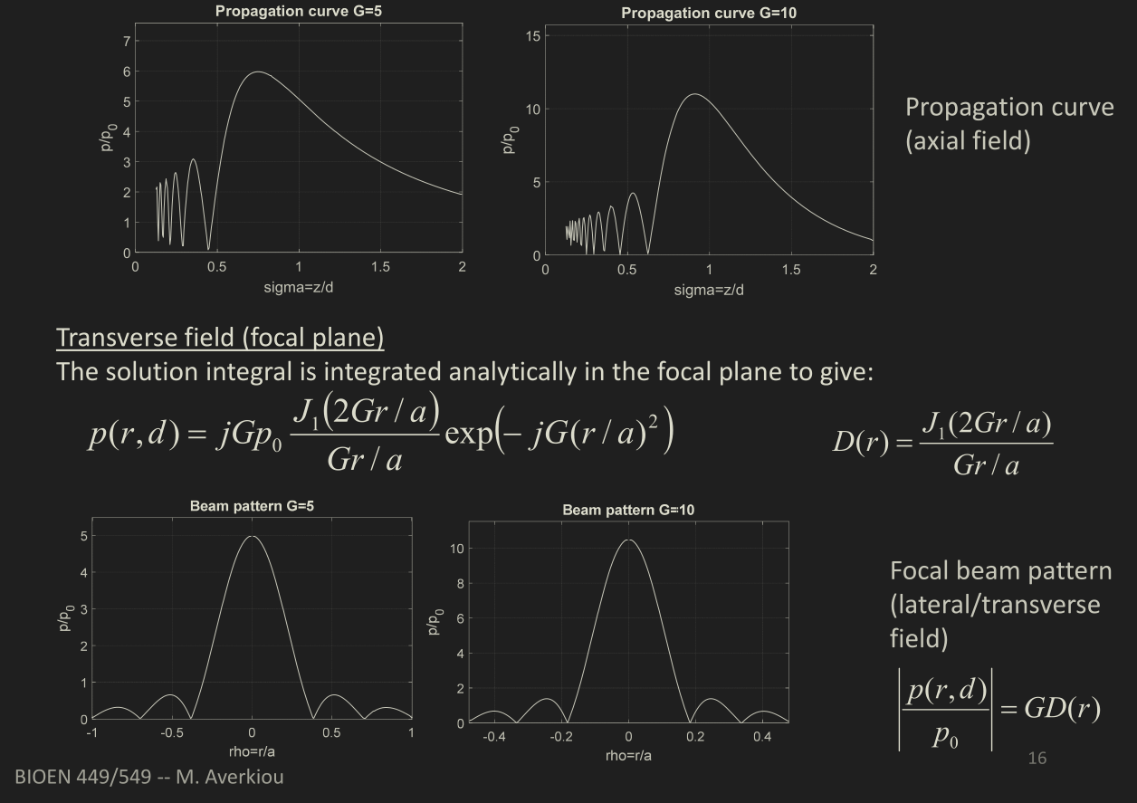
Focused beams

Sound beams for biomedical applications

1. Size: 1-10 cm dia or side, 1-20 cm focus
2. Frequencies: 0.5-10 MHz.
3. Medium: blood, soft tissues.
1. Density: 1000 kg/m^3
2. Speed of sound: 1500 m/s.
3. Attenuation: ~0-1 dB/cm/MHz .

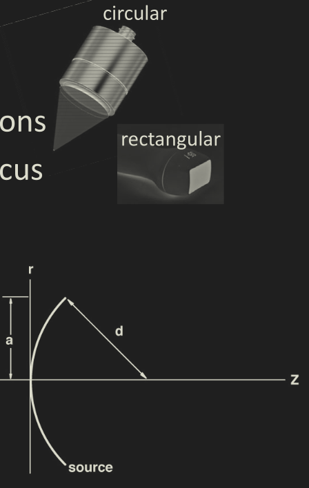
Focused beams

1. Focusing implemented with either curved transducers, a lens, or electronics delays
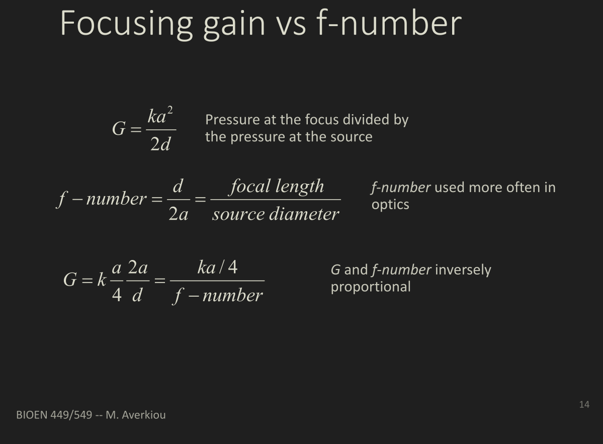
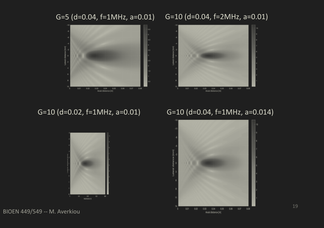
2. Focusing gain: pressure at focus dividied by the pressure at the source.
3. \( G = \frac{p(x=d)}{p(x=0) }=\frac{ka^2}{2d} \)

Unfocused beams

Near field directing of beam:

Focused beams

Shallow focus:

Focused beams

Deeper focus:

Single slit diffraction pattern (rectangular aperture)

\( P(r) = A(r)e^{j \omega t} (e^{j k r_1} + e^{j k r_2} + ... + e^{j k r_N}) \)

\( r_2 = r_1 + d \sin \theta \\ r_3 = r_1 + 2d \sin \theta \\ ... \\ r_N = r_1 + (N-1)d \sin \theta \\ \)

\( P(r) = A(r)e^{j \omega t} e^{j k r_1} S \)

\( S = 1 + e^{j k (r_2 - r_1)} + e^{j k (r_3 - r_1)} + ...\)

\( S = 1 + a + a^2 ... a^{N-1}\)

Single slit diffraction pattern (rectangular aperture)

\( S = 1 + a + a^2 ... a^{N-1} \)

\( a = e^{j k (r_2 - r_1)} = e^{jk \sin \theta}=e^{j \Delta \phi} \)

\( \Delta \phi = k d \sin \theta = \frac{2 \pi}{\lambda }d \sin \theta \)

\( aS - S = a^N - 1 \)

\( S = \frac{a^N-1}{a-1}\)

Single slit diffraction pattern (rectangular aperture)

\( aS - S = a^N - 1 \)

\( S = \frac{a^N - 1}{ a - 1} = \frac{e^{jN \Delta \phi} - 1}{ e^{j \Delta \phi} - 1} = \frac{e^{j(1/2)N \Delta \phi}}{e^{j(1/2) \Delta \phi}} \frac{e^{j(1/2)N \Delta} - e^{j(1/2)N \Delta}} {e^{j(1/2) \Delta} - e^{j(1/2) \Delta} } \)

\( S = e^{jN \Delta \phi} \frac{\sin \frac{1}{2} N \Delta \phi}{\sin \frac{1}{2} \Delta \phi} \)

\( N \to \infty, \; \; \; \Phi =(N-1)\Delta \phi = kD \sin \theta \)

\( \Phi \approx N \Delta \phi \)

\( S = \frac{\sin \frac{1}{2} \Phi}{\sin \frac{1}{2} \Phi / N}= \frac{\sin \frac{1}{2} \Phi}{\frac{1}{2} \Phi } \; \; \; \; \Phi = 2 \pi \frac{D \sin \theta}{ \lambda }\)

\( \Delta \theta = \frac{\lambda}{D} \)