Current Projects: Threshold Wind Speeds

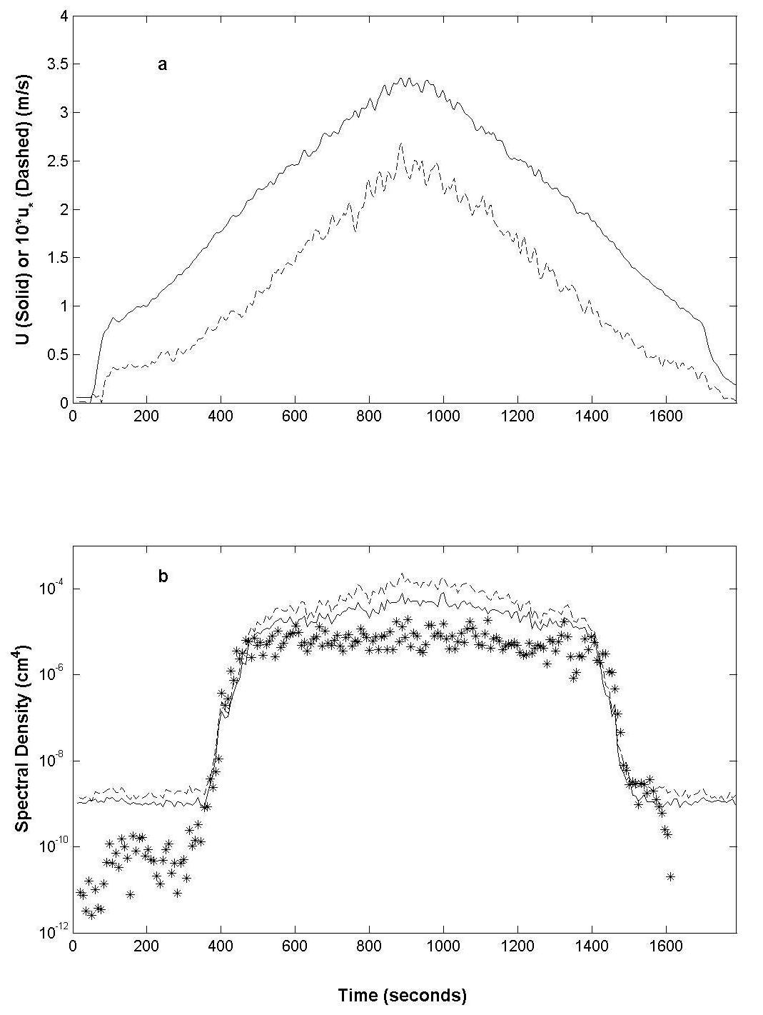
INTRODUCTION

Several experiments we have conducted clearly show that gravity-capillary waves do not appear on the sea surface until momentum transfer from the wind can overcome viscous damping.   This implies that a threshold wind speed exists for any measurement that responds to the amplitudes of these short surface waves.  We have observed threshold effects in microwave backscatter in wind wave tanks, in microwave backscatter from the ocean observed from an airship, and in NSCAT scatterometer data.  The most definitive study (Donelan and Plant, 2002) of this threshold effect has been our comparison of microwave backscatter in a wind wave tank with surface wave spectra determined by Mark Donelan of the University of Miami using his wavelet technique applied to laser wave gauges (Donelan et.al., J.Phys. Ocean. 26(9), 1901-1914, 1996)..

THRESHOLD WIND SPEEDS IN WAVETANK MEASUREMENTS

For measurements in a wind wave tank with the wind speed slowly ramping up, both radar and laser probes show that short waves do not begin to grow until the wind speed reaches a threshold value (Figure 1).  Note that thresholds occur both as the wind ramps up and as it ramps down.

Figure 1. a) Time plot of wind speed at 3 cm (solid line) and friction velocity at the surface (dashed line) for a slowly ramped wind (ramp rate = 0.34 cm/s/s). b) Time plot of F(k_b,0) from Ku band radar cross sections and F(k_b,0) from the laser height/slope gauge, where k_b = 335 rad/m. The radar antenna was at a 35^o incidence angle looking upwind. The fetch at the radar footprint was 10.0 m while the fetch was 14.3 m to the laser probe. Solid curve - radar, VV; dashed curve - radar, HH; asterisks - laser.

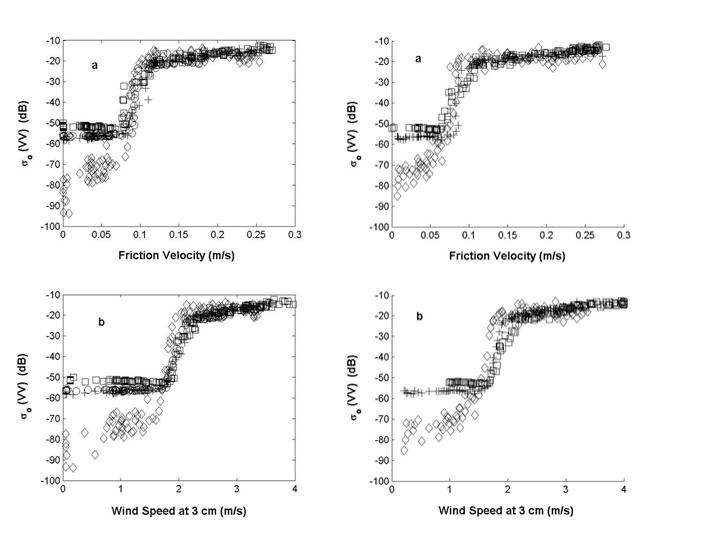
Plotting microwave cross section versus friction velocity or wind speed shows that the threshold wind speed is different for the up ramp than for the down ramp (Figure 2)

Figure 2. Left - Ku band cross sections, σ_o, at different fetches for a slowly increasing wind  versus (a) friction velocity and (b) wind speed at 3 cm. Rate of change of wind speed is 0.3 cm/s/s. Symbols are as follows: squares = σ_o(VV), downwind, 7.4 m fetch; pluses = σ_o (VV), upwind, 10.0 m fetch; circles = σ_o(VV), downwind, 12.4 m fetch; diamonds = spectral densities from laser converted to σ_o (VV), 14.3 m fetch. Radar is at a 45^o incidence angle, k_b = 415 rad/m.  Right - Ku band cross sections at different fetches for a slowly decreasing wind versus (a) friction velocity and (b) wind speed at 3 cm. Rate of change of wind speed is 0.3 cm/s/s.

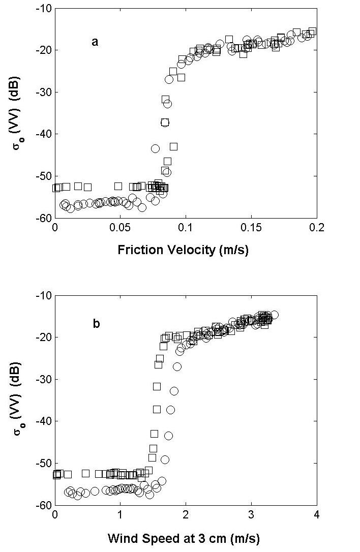
Increasing the water temperature decreases the wind speed threshold but not the friction velocity threshold (Figure 3).  The friction velocity adjusts to the changing conditions on the water surface.

Figure 3. Ku band radar cross sections, σ_o, at two different water temperatures for a decreasing wind versus (a) friction velocity and (b) wind speed at 3 cm. Data taken at a fetch of 10.0 m with an upwind look direction; incidence angle is 45^o (k_b= 415 rad/m). Rate of change of wind speed is 0.3 cm/s/s. Air temperatures were between 20^oC and 22^oC. Symbols indicate water temperature as follows: circles = 20.0^oC, squares = 29.4^oC.

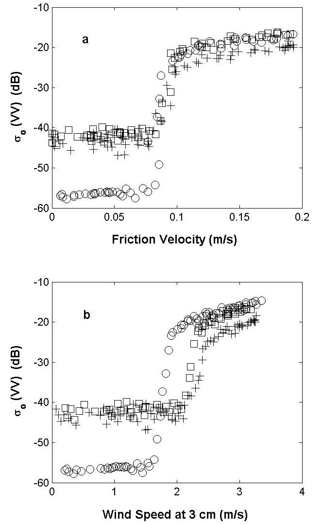
Similarly, changing current in the water changes the wind speed threshold but not friction velocity threshold (Figure 4).

Figure 4.  Ku band radar cross sections with different currents and a decreasing wind versus (a) friction velocity, and (b) wind speed at 3 cm. Rate of change of wind speed was near 0.3 cm/s/s, air temperatures were about 22^o, and water temperaures were between 18^o and 21^o. Symbols indicate different currents as follows: circles = 0 cm/s, squares = 12 cm/s, pluses = 27.6 cm/s. The antenna was directed upwind for the two lower currents (fetch = 10.0 m) and downwind for the higher (fetch = 7.4 m); the incidence angle was 45^o (k_b = 415 rad/m).

Further information about these experiments can be found in Donelan and Plant, 2002.

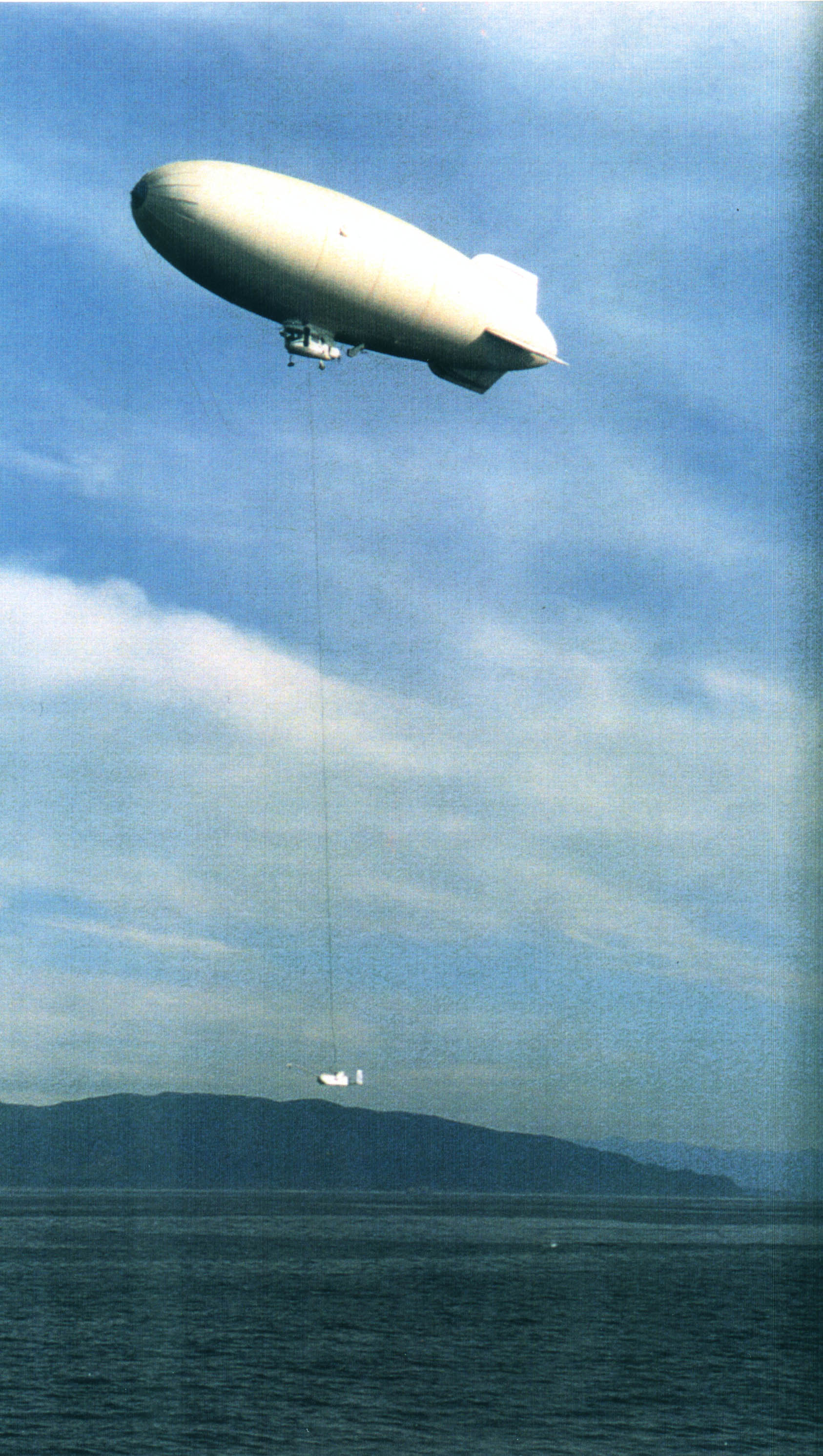
THRESHOLD WIND SPEEDS IN AIRSHIP MEASUREMENTS

We made measurements from an airship using a Ku-band microwave system.  Figure 5 shows the airship in flight with our equipment on board.

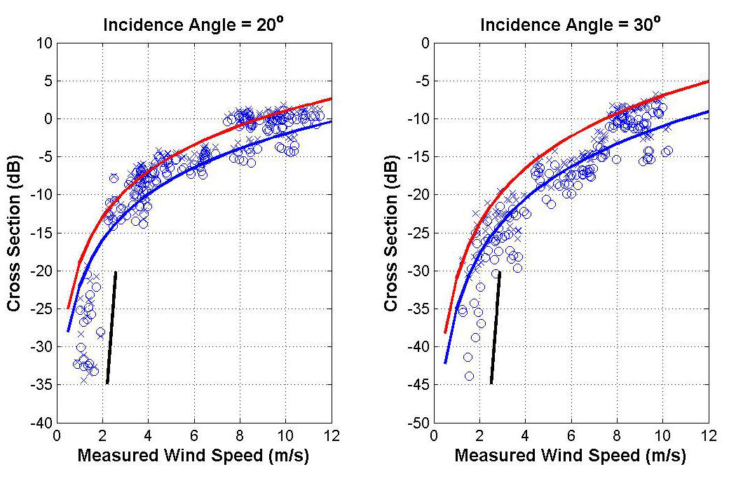
Figure 5.  The US-LTA Model 138S airship with the suspended meteorological platform of the Naval Research Laboratory below it.  APL/UW's Ku-band microwave system is mounted in the gondola of the airship.

Measured Ku-band cross sections plotted versus wind speed showed a threshold wind speed somewhat below that predicted by Donelan and Pierson, JGR, 92(C5), 4971-5030, 1987 (Figure 6).  The reason that the measured threshold is below the predicted one is due to the variability of the wind over the measurement time.  This variability reduces the impact of the threshold wind speed on spaceborne scatterometer measurements as shown in the next section.

Figure 6. Azimuthally averaged 14 GHz cross sections versus measured wind speed for two different incidence angles. Wind direction was required to vary by less than 15^o in one minute. Curves are power laws drawn through arbitrarily chosen regions of high and low cross sections. Straight lines are low-wind-speed cross sections predicted by Donelan and Pierson at our water temperatures.

THRESHOLD WIND SPEEDS IN NSCAT SCATTEROMETER CROSS SECTIONS

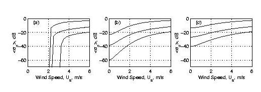
The NSCAT scatterometer, a Ku-band spaceborne instrument, received backscatter from the ocean surface from a footprint approximately 6 km by 25 km in size.  If the wind varies over this footprint, the threshold wind speed found in wave tank measurements gradually ceases to be obvious.  This is shown in Figure 7. 

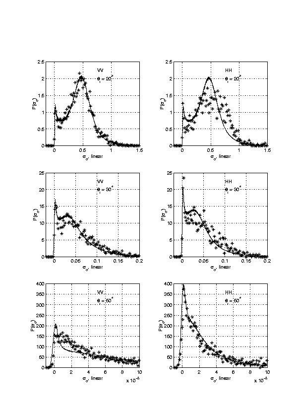
Figure 7.  Model functions corresponding to Ku-band VV polarization, an upwind antenna look direction, and incidence angles of 20^{\circ}$, 30^{\circ}$, and 50^{\circ}$. a) The zero-variance model function, NSCAT2 with a threshold wind speed. b) The model function  with a wind speed variance of  0.9 m/s. c) The  model function with a wind speed variance of 1.4 m/s.

Even when the model function is smoothed by wind variations, a higher probability of measuring very low cross sections exists than in the case of a model function with no threshold.  This make threshold wind speed effects visible in probability density functions of backscattered cross sections.  An example is shown in Figure 8 where probability density functions of NSCAT's cross sections at three different incidence angles are shown.  The spikes in the distribution at zero cross section do not occur if the model function does not display a threshold.  More information can be found in Plant, JGR, 105, 2000.

Figure 8.  Probability distribution of σ_ocollocated with TAO buoys in the equitorial Pacific. The various plots are for various polarizations and incidence angles θ_i as indicated. Asterisks are NSCAT data. Solid lines are predictions of theory using the NSCAT2 model function with a low wind speed threshold but averaged over a wind vector distribution with a variance of 0.9 m/s.