This research was sponsored by the Remote Sensing Program of the Office of Naval Research.
![]()
INTRODUCTIONOur research has shown that in addition to freely propagating short wind-generated waves the ocean surface contains a significant population of bound waves. These are waves that are not generated directly by the wind but rather are produced by longer waves. Bound waves may be simply nonlinear distortions of the longer waves, parasitic capillaries on the front faces of the longer waves, or turbulence generated by the breaking of the longer waves. We have noted effects of bound waves both in wind wave tanks and on the ocean. In tanks, the influence of bound waves on simultaneous microwave and acoustic surface scattering is detectable in their different levels of return. Also, mean Doppler shifts observed in many tank settings are larger than could be produced by free waves, again indicating the presence of bound waves. On the ocean, the different Doppler shifts evident in HH and VV polarized Doppler spectra can be explained on the basis on bound waves. Finally, bound waves can explain sea-surface slope probability density functions observed in optical measurements of sun glitter patterns.
BOUND WAVES EFFECTS IN BACKSCATTER PARASITIC WAVE EFFECTS ON MICROWAVE AND ACOUSTIC BACKSCATTER IN A WAVETANK In the wind wave tank at the University of Washington, we arranged to view the same spot on the water surface with microwaves from above and acousitc radiation from below. We arranged that the two systems, radar and sonar, viewed the surface at the same incidence angles and that their transmitted wavelengths were within 10% of each other. This made the Bragg resonant wavelengths for microwave and acoustic backscatter lie within 10% of each other and we utilized both 0.8 and 2 cm radiation. We found that for the 0.8 cm radiation, HH polarized microwave cross sections were 10 to 15 dB larger than acoustic ones when both systems looked upwind. When the radar viewed the water in the upwind direction and the sonar looked downwind, however, these cross sections were nearly the same. This is shown in columns (b) and (c) of Figure 1.
Figure 1. Polarization ratio σo(VV)/σo(HH) of the microwave backscatter (left column) and the ratio of HH radar cross section to sonar cross section (middle and right columns) plotted against incidence angle at various wind speeds. The middle column corresponds to the acoustic transducers looking upwind, while the right column shows ratios with the acoustic system looking downwind. Curves are the predictions of Bragg scattering theory. We found that this behavior could be explained very easily by supposing that Bragg scattering was taking place from surface waves whose mean slope was not zero. Figure 2 diagrams the model. The observed cross section ratios can now be easily explained. When both systems looked upwind, the local incidence angle at the location of the tilted short waves shown in the figure is smaller than that of the sonar when it looks upwind. Hence the higher cross sections for the radar in this configuration. When the sonar looked downwind, the local incidence angles were the same so the cross sections were nearly identical. The lines in Figure 1 show how well Bragg scattering with this model explains the data.
Figure 2. Schematic illustrating the surface wave model used to account for the scattering reported here. Note that at the location of the parasitic capillaries on the front face of the parent wave, the radar incidence angle is lower than that of the sonar when it is directed upwind.
We postulated that the bound, tilted waves that were acting as scatterers for the microwave and acoustic radiation were in fact the parasitic capillaries that had been known both experimentally and theoretically for many years. One characteristic of these parasitic capillaries is that they move at a speed that is both their intrinsic phase speed and the phase speed of the long, parent wave. Figure 3 shows that our scatterers satisfy this criterion.
Figure 3. Doppler offsets f1 for the two microwave polarizations and for the acoustic system looking upwind as a function of incidence angle at various wind speeds. Solid lines are the predictions of Bragg scattering theory for a scatterer moving at the phase speed of the dominant wave in the tank. Dashed lines are similar predictions for freely propagating capillary waves. (a) circles = VV polarization; asterisks = HH polarization; lines = both polarizations. (b) Acoustic upwind. . Spectral densities deduced from the backscatter cross sections also agree with those expected for parasitic capillary waves. More details of this project can be found in Plant et.al., JGR, 104, 1999.
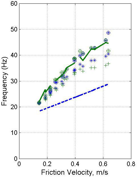
OTHER BOUND WAVE EFFECTS ON MICROWAVE BACKSCATTER IN WAVE TANKS For lower microwave frequencies, the Bragg waves are too long to be parasitic capillary waves. Yet our measurements in both the wave tank of the Canada Centre for Inland Waters (CCIW) and the wide tank at Luminy, France show that many of the scatterers move too fast to be freely propagating wind waves. Figure 4 shows measurements of the peak of the Ku-band Doppler spectrum and its first moment compared with frequencies expected if the Bragg waves travels at its own phase speed and if it travels at the phase speed of the dominant wave in the tank. The figure clearly shows that the peak of the Doppler spectrum is due to a scatterer moving at the phase speed of the dominant wave in the tank but that the first moment is lower. This shows that both free and bound waves exist in the tank but that the backscatter from the bound waves exceeds that of the free waves. Additional information on these experiments can be found in Plant et.al., JGR, 104, 1999.
Figure 4. Microwave backscatter data taken in the CCIW tank at a 45o incidence angle looking upwind on April 14, 1993 versus friction velocity. The figure shows the peak frequency, fp, and first moment, f1, of the Doppler spectra. Asterisks = f1, HH; + = f1, VV; circled asterisks = fp, HH; and circled + = fp, VV. The solid line is the shift expected from a scatterer travelling at the dominant wave phase speed and the dashed line is the shift due to a free Bragg scatterer. The existence of both types of waves on the surface is perhaps more clearly shown in Doppler spectra collected at Ku-band in the Luminy tank. Figure 5 shows spectra collected with a radar and sonar aligned as described above with both looking upwind.
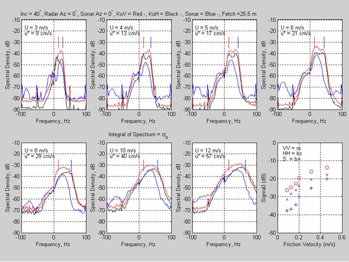
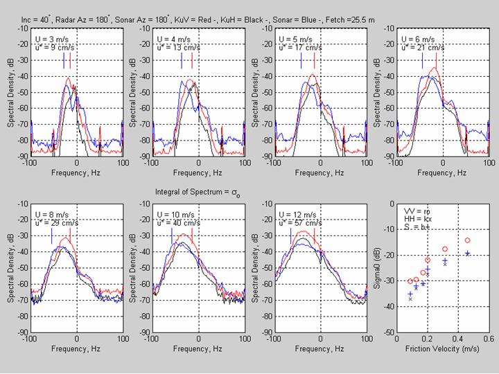
Figure 5. Top - A series of Doppler spectra from radar and sonar at a variety of wind speeds looking upwind. Last panel shows cross section versus friction velocity. Bottom - A series of Doppler spectra from radar and sonar at a variety of wind speeds looking downwind. Last panel shows cross section versus friction velocity. Short blue vertical lines show the Doppler shift expected from a Bragg wave traveling with the dominant wave in the tank. Short red vertical lines show the Doppler shift expected from a Bragg wave traveling at its intrinsic phase speed.
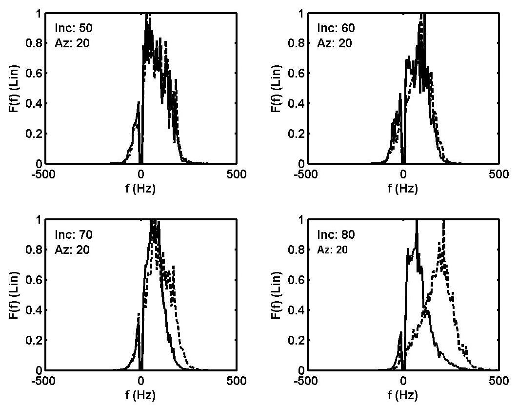
BOUND WAVE EFFECTS ON MICROWAVE DOPPLER SPECTRA OF SEA RETURN AT HIGH INCIDENCE ANGLES When examining data taken during ONR's SAXON-FPN Phase II in 1991, we observed that HH and VV polarized Doppler spectra were shifted by different amounts when viewing the sea surface at relatively high incidence angles. This difference did not occur at moderate incidence angles. The four left panels of Figure 6 give an example of this behavior for Ku-band data taken at a wind speed of 7 m/s with the antenna looking nearly into the wind.
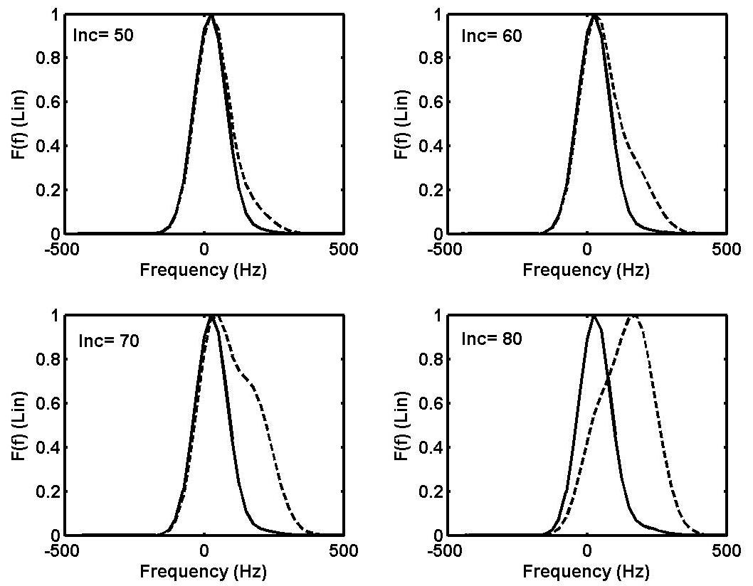
Figure 6. Doppler spectra of Ku-band sea return. The left four panels are data collected during SAXON-FPN Phase II. The right four panels are modeled spectra using a bound wave / free wave model as shown in Figure 7. We also found in looking at this data that dominant wave spectra could not be obtained from the motion of the centroid of the Doppler spectrum for spectra taken at high incidence angles. At moderate incidence angles, this is a well-known technique for obtaining ocean wave spectra. We found that both of these observations could be modeled reasonably well with a bound wave / free wave model for the short waves on the surface. A schematic of the model is shown in Figure 7. The model is that very long waves on the ocean modulate the amplitudes and frequencies of waves of an intermediate scale. At some phase of the long waves, these intermediate waves become sufficiently steep due to this modulation that they break or "crumple". This creats bound, tilted waves that move along at nearly the phase speed of the intermediate waves. These bound, tilted waves show up more in HH backscatter at high incidence angles than in VV because backscatter from the free waves at HH drops to very low values, allowing observation of the bound waves. This accounts for the differential doppler shift observed in Doppler spectra at the two polarizations. More information can be found in Plant, JGR, 102, 1997.
Figure 7. Diagram of sea surface model used to explain Doppler shifts in microwave sea return at high incidence angles. Long waves modulate intermediate waves to the point of breaking at some phase of the long wave. This produces bound, tilted waves traveling with the intermediate waves.
BOUND WAVES IN SLOPE PROBABILITY DENSITY FUNCTIONS
EFFECTS ON SURFACE SLOPE PROBABILITY DENSITY FUNCTIONS IN WAVETANKS Working with us in a wind wave tank at the Canada Centre for Inland Waters, Mark Donelan measured surface slope probability density functions (PDFs) using a laser slope gauge as part of our joint studies of wind-generated waves and microwave backscatter. Figure 8 shows examples of these PDFs for two different wind speeds and for upwind and cross wind slopes.
Figure 8. Histograms of slopes measured in the CCIW wave tank. Open circles represent histograms of uptank and crosstank slopes normalized to one at the peak. The dashed line is a Gaussian fit to slopes higher than the peak of the histogram extended below the peak. The thin solid line is a Gaussian fit to the dots which are obtained by subtracting the dashed line from the open circles. The thick solid line is the sum of the dashed and thin solid lines, which is our best fit to the data. We interpret the dashed line to be the best fit to the histogram of free waves, the thin solid line to be the same for bound waves, and the thick solid line to be this fit for the total slopes. Note that the bound waves were not found in the crosstank slopes. Clearly the overall PDFs for upwind slopes consist of the sum of two Gaussian PDFs of different probabilities. One of the Gaussians has a mean slope very different from zero and we identify this PDF with bound waves that are riding on the forward face of longer waves. This is as expected from Bayes' Theorem which states that if only free and bound waves exist on the surface then the overall PDF may be expressed as a sum of weighted conditional PDFs: P(s) = Pf P(s|f)+Pb P(s|b). As seen above, this dichotomy between bound and free waves is able to explain many features of microwave and acoustic scattering in tanks and at sea. For more information see Plant et.al., JGR, 104, 1999.
EFFECTS ON SEA-SURFACE SLOPE PROBABILITY DENSITY FUNCTIONS We have re-examined the sea-surface slope PDFs measured by Cox and Munk using sun glitter patterns (Cox and Munk, Deep Sea Research, J. Mar. Res., 13(2), 1954.) As in the tank, these PDFs can be fit well by a sum of Gaussian PDFs having different weights. This is shown in Figure 9.
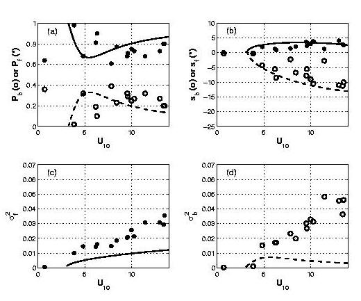
Figure 9. Comparison of Cox and Munk's sea-surface slope PDF fits with a Gram-Charlier series and with a free/bound wave model. The solid curve is the Gram-Charlier fit, the squares are Pf times the free-wave PDF, the circles are Pb times the bound-wave PDF, and the asterisks are the sum of the circles and squares. The wind speed at 12.5 m height was 13.5 m/s for this PDF. The existence of bound waves is not as evident on the ocean as it is in the tank due primarily to the larger variances of the individual Gaussian PDFs. This is shown by a comparison of parameters necessary to fit PDFs at sea with those in a wave tank. This comparison is shown in Figure 10.
Figure 3. Bound and free wave parameters versus wind speed at 10 m height. Symbols were deduced from fits to the Cox and Munk (1954, 1956) data and therefore represent ocean data. Solid curves show best fits to results obtained in a wind wave tank (Plant et.al., JGR, 104, 1999). (a) Probability of finding bound or free waves. (b) Mean slopes of bound and free waves. (c) Variance of free waves. (d) Variance of bound waves. More information on this study can be found in Plant, 2003.
|