Spin Simulation for Magnetic Resonance Force Microscopy (MRFM)

Jon Jacky, March 2005

Magnetic Resonance Force Microscopy (MRFM)

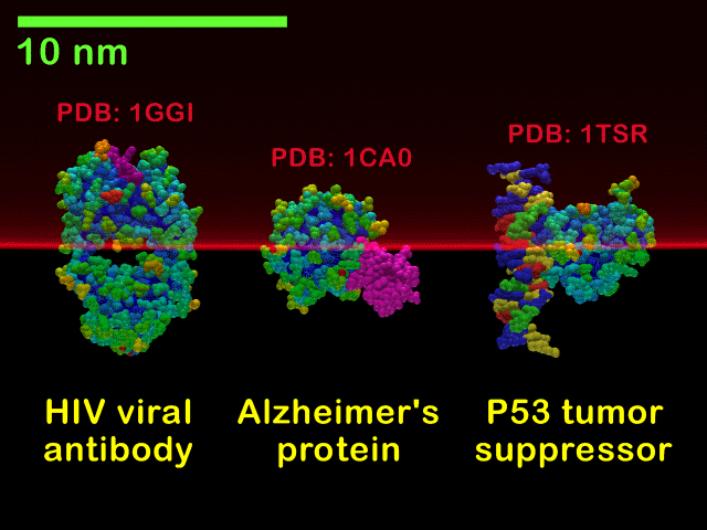
Goal: molecular microscope, 3D images of individual molecules in situ

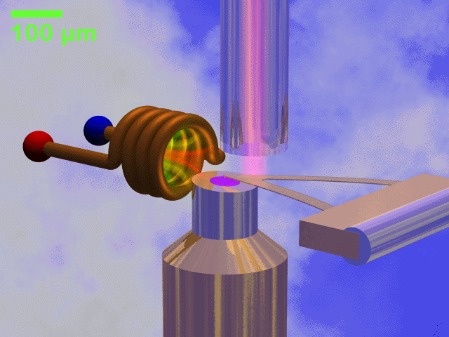
Marriage of atomic force microscope (AFM) and MRI imaging

Spins in sample excited by RF exert magnetic force on cantilever, detected by interferometer.

Scan sample past cantilever (or vice versa), deconvolve signal to obtain 3D image.

Invented/developed here at UW School of Medicine and UW Dept. of Mechanical Engineering by John Sidles, Joe Garbini, et al.

RF coil (left), sample positioner (bottom), interferometer (top), cantilever (right)

Cantilever tip with permanent magnet, showing resonant slices due to magnetic field gradient. At a given RF, spins in only one slice exert force on the cantilever.

Molecules in a resonant slice

Purpose

Purpose of simulation

Predict signals and noise expected from molecules of interest: how long does it take for spins to lock to RF, etc?

Investigate coupling between spins in the sample: significant effects?

Purpose of this study

Investigate MPI-style parallel programming techniques and performance in this application.

Spin dynamics

dvi/dt	=	b_toti X vi (vector cross product)
b_toti	=	b_rfi + Sum (all other j) Bij vj (matrix-vector product)

B_ij describes coupling between spins i and j
B_ij is characteristic of the sample (particular molecule), parameter (input) to simulation

Due to coupling between spins, might be lots of communication --- maybe too much!

Expect computation time proportional to number of interactions, N²

Output is v(t) for all v_i, t = 0 1 2 ... tn, tn is 1000s or 10000s

Integration

Integrate a system of ODEs

dv_i(t)/dt = b_tot X v_i(t)

Euler integration: straight-line extrapolation using present rate of change.

v_i(t+1) = v_i(t) + dt * dv_i(t)/dt

Runge-Kutta integration: weighted average of Euler estimates at different t, dt

We use 4th order Runge-Kutta (4 estimates)

Parallelization

Intuition: each process simulates one spin (or n spins)

N spins, np processes, n = N/np spins/process

Each process just computes, updates one (or n) v_i

Due to coupling between spins, each process must read all v_j, use all relevant B_ij

All updated v_i must be distributed to all processes after each time step

In each time step, communication proportional to N, computation proportional to N²

Expect advantage of parallelization to grow with N

BUT there must be an upper limit to the number of significantly interacting spins, independent of N: about 20 or 30 nearest neighbors, we expect.

Program

From scratch, by hand (C and MPI only, no other libraries)

Obvious (naive?) coding: for (i=0;i<n;i++) for (l=0;l<3;l++) v[i][l] = ...

Three stages: read, compute, write. No file I/O during compute stage.

1. Read: front end node reads all initial v_i and all B_ij, Broadcast
2. Compute: loop for each time series point
   In each process ---
     Compute all n v_i(t+1) from v_i(t) and all N v_j(t)
     Add v_i(t+1) to time series in process memory
     Allgather v_i(t+1) from each processor
   Do 4 of these Runge-Kutta substeps for each time series step
3. Write: Gather time series, front end node writes file.

Performance experiment

Two test cases: large and small number of spins N = 160, 32. Measure performance of each case on different numbers of processors np = 1,2,4,8,16,32.

Number of spins N and number of time steps tn chosen to take appreciable but not overwhelming time, so timing measurements meaningful. Here is the elapsed time of both cases on a Mac G4 with one processor:

N	N2	tn	elapsed	(CPU)	Comment
160	25,600	1000	26 sec	(26)	Large N, parallel advantage expected
32	1024	25000	25 sec	(20)	Typical number of interactions expected

Not a real molecule, arbitrary (random) initial spins and coupling matrices

Measure multiprocessor performance on ladon cluster. Report elapsed (wall) time and computation (CPU) time (on one CPU) for computation stage only (quite reproducible, unlike read and write) Also report elapsed time only for read and write stages. Elapsed times are in seconds.

With N = 160, the program is pleasingly parallel. Doubling np almost doubles speed up through 8 processors (but little or no improvement after that).

np	N	tn	read	elapsed	(CPU)	write
1	160	1000	0.28	16.66	(16.62)	5.23
2	160	1000	0.40	9.41	( 8.81)	5.074
4	160	1000	0.47	6.08	( 4.16)	9.36
8	160	1000	0.48	3.53	( 1.84)	18.26
16	160	1000	0.72	3.38	( 1.28)	7.77
32	160	1000	1.00	3.45	( 1.50)	11.09

With N = 32, the program is pathological. Adding processors slows it down!

np	N	tn	read	elapsed	(CPU)	write
1	32	25000	0.01	6.86	(6.83)	26.44
2	32	25000	0.02	13.45	(7.03)	48.20
4	32	25000	0.02	22.27	(8.70)	105.03
8	32	25000	0.02	37.84	(12.07)	182.63
16	32	25000	0.34	46.28	(17.82)	330.42
32	32	25000	0.27	60.65	(28.39)	430.11

Conclusions

One processor is enough for small and medium-sized simulations: we can simulate 1000 interactions/msec (~30 spins) on a Mac G4.

The same program can be pleasing or pathological depending on just one parameter; cutover point is hard to predict.

Underwhelming benefit from parallelism in this program, for the two cases tested.

Future work

Investigate better parallelization strategy.

Consider 100s or 1000s of spins, where each interacts with ~20 neighbors.

Pre-compute lists of neighbors where interaction matters.

Optimize communications (processes on virtual 3D grid, communicate only with neighbors).

Investigate speeding up serial computation. Vectorization (SSE for x86, Altivec for G4) promises up to 4x speedup (vs 8x found for parallelization).

Visualization (show spins coupled to cantilever)