These MATLAB data files contain the sound speed, temperature, salinity, buoyancy profiles for the world's oceans derived from the 2001, 2005, or 2009 World Ocean Atlases (World Ocean Atlas, or the alternate ftp site). Sound speed was calculated from annual mean temperature, salinity and pressure using the Del Grosso sound speed equation. The World Ocean Atlas is at 1-degree resolution. All profiles were then extended to 5500-m depth using nearest-neighbor values, and extended to all points the world over at 1-degree spacing, similarly. Variables are given at places where there is land to make the interpolation to arbitrary points easier (e.g., cubic splines for points near continents can go beserk otherwise). Curiously, this means you can calculate acoustic propagation times from Vladivostok to Berlin; the user is expected to know where the water ends and the dirt begins. Note that these files are a subset of the complete WOA. Information as to the hydrographic sampling, statistics, and other variables, and monthly and seasonal values, are all part of the complete WOA.
To compress the data file, the sound speed values in the MATLAB file have had 1000 subtracted from them, then multiplied by 100, and then rounded to the nearest integer, e.g., 1478.32 is saved as the integer 47832. Other variables are multiplied by 1000 and rounded to the nearest integer, e.g., 25.346 goes to the integer 25346. This makes the MATLAB files have the highly compressed size of 4.3 MB. The trade off is that sound speed is good to the nearest hundredth of a m/s, while other variables are good to the nearest thousandth. An additional MATLAB file stores the latitudes, longitudes and depths of the WOA.
Download the 2001 data files and put them in a convenient directory
(in Netscape,
Sound Speed (lev_ann.mat - 4.3 MB)
Temperature (levT_ann.mat - 4.3 MB)
Salinity (levS_ann.mat - 4.3 MB)
Buoyancy (levN_ann.mat - 4.3 MB)
The Latitude, Longitude, Depth file (lev_latlonZ.mat - 260 KB).
NEW! The 2009 WOA is available now, and converted to t he same matlab format as above. Download the tarball of *.mat files from: WOA 09. The 127 MB tar ball includes files for temperature, salinity, sound speed, and buoyancy, and it includes data files for annual, seasonal and monthly atlases. N.B.#1: It has been reported that Windows/winzip corrupt matlab's *.mat files when they are unpacked from a tarball. N.B.#2: These *.mat files were saved using matlab version 2010b; older versions of matlab may not be able to load these files.
The 2005 WOA was also converted to the same matlab format as above. Download the tarball of *.mat files from: WOA 05. The 115 MB tarball includes files for temperature, salinity, sound speed, and buoyancy, and it includes data files for annual, seasonal and monthly atlases. N.B.#1: It has been reported that Windows/winzip corrupt matlab's *.mat files when they are unpacked from a tarball. N.B.#2: These *.mat files were saved using matlab version 7; older versions of matlab may not be able to load these files.
A few associated MATLAB scripts can be used to extract the variables at arbitrary
points and write out a data file. These are a few programs borrowed from our
MATLAB acoustic propagation gui package.
getlev.m - the driver program. Modify a line near the top of this program to set the data file directory.
getLevSSPs.m - the engine.
dist.m - a generic program for computing distance and bearing between points on the earth using various reference spheroids. A program having a long sordid history beginning with Peter Worcester in the early '80's and ending with Rich "Mr. Matlab" Pawlowicz.
EXAMPLE: Here is a small example of how you might use these data/scripts in MATLAB. The scripts are certainly not professionally polished - please adapt them for your own purposes.
> lat=[22 30];
> lon=[-70 -60];
[These are two positions in the North Atlantic. The programs will secretly convert the negative longitudes to positive longitudes by adding 360; this is something to be a little careful about. The negative values will be returned.]> [r, glat, glon]=dist(lat,lon,50);
[Get 50 points on a path between the two positions (WGS 1984 is the default).]> [P1,z]=getlev(glat,glon,'c');
> [P2,z]=getlev(glat,glon,'T');
[Gets the World Ocean Atlas sound speed (P1) and temperature (P2) profiles (at the 33 standard depths) on those 50 points and writes them to a file "templev.ssp". (The file is overwritten by the second call). Sound speed and depth are reported back in P1 and z, respectively. P1, P2 are 33X50 matrices.]> figure(1); plot(P1,-z/1000); xlabel('Sound Speed (m/s)'); ylabel('Depth (km)')
> figure(2); plot(P2,-z/1000); xlabel('Temperature \circC'); ylabel('Depth (km)')
> figure(3); contour(glon,-z/1000,P2); xlabel('Longitude'); ylabel('Depth (km)'); title('Temperature')
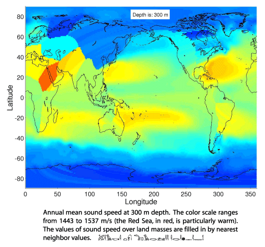
Here is a color map of sound speed at 300 m depth. It shows the effects of filling in sound speed values over land masses by nearest-neighbor values. The code fragment to make this figure, which will also show the format of the data files, is:
> load lev_ann.mat [Loads in c]
> load lev_latlonZ.mat [Loads in lat, lon, z]
> lat1=reshape(lat,360,180)*0.1;
> lon1=reshape(lon,360,180)*0.1;
> % depth 12 is 300 m
> cc=1000+reshape(c(:,12),360,180)/100;
> surf(lon1,lat1,cc); shading flat; view([0 90])